MIR views: tempogram and chromagram

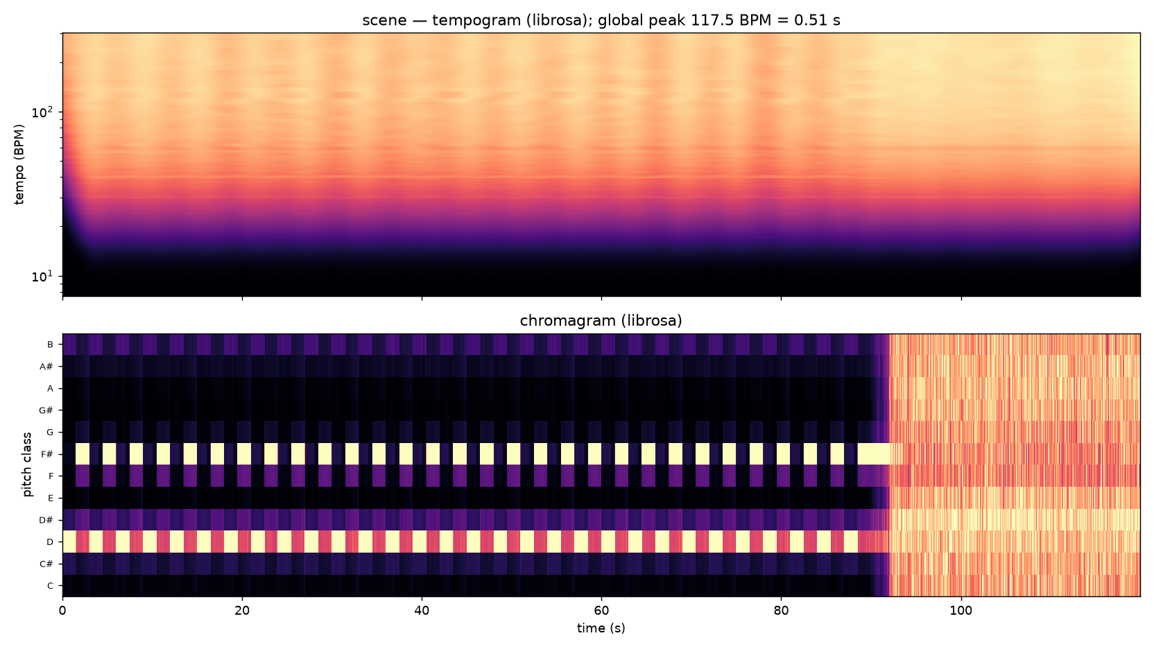
ambiscape music adds the two standard music-information-retrieval views on top of the built-in analyses: the tempogram (onset autocorrelation over time, in BPM) and the chromagram (12-bin pitch-class energy over time). They are the time-resolved, MIR-conventional counterparts of the built-in rhythm tempogram and tonality.pitch_class_profile, useful as an independent cross-check and for readers who expect the librosa picture.

ambiscape music <session-folder> --t0 60 --dur 1500   # needs the [music] extra

Reads audio directly (not the feature cache), so it needs pip install "ambiscape[music]". --t0 and --dur (seconds into the first take) bound the analysed span; a 25-minute file takes on the order of a minute. Analysis runs on the mono W reference resampled to 22.05 kHz.

Writes music.json (tempo_bpm_global and tempo_period_s from librosa's global tempo estimate, chroma_mean — the 12 pitch classes normalised to sum to 1 — and top_pitch_classes) and music.png (the tempogram over the chromagram).

In Python

from ambiscape import music

y, sr = music.load_w(sess.takes[0], t0=60, dur=1500)
times, bpm, T, tempo = music.tempogram(y, sr)   # T is the tempogram matrix
tc, C = music.chromagram(y, sr)                 # C is 12 x n_frames

tempogram returns librosa's global tempo alongside the matrix, which resolves the octave ambiguity a raw tempogram argmax suffers from. Because this is the MIR-standard estimator, a disagreement with the built-in rhythm tempo is diagnostic rather than an error — the two use different onset models.

Circular views: pulse clarity and the circle of fifths

Three functions apply the circular statistics machinery to musical material. They were developed on a five-album solo-harp catalogue (57 tracks) where conventional beat tracking fails outright.

music.pulse_clarity(y, sr)
# {"R": 0.05, "period_s": 0.47, "period_bpm": 127.7, "rayleigh_p": ..., "n_onsets": 412}

pulse_clarity measures metric lock rather than tempo: onsets are folded at the dominant period and the strength-weighted resultant length R taken as the score — 0 is free rubato, 1 metronomic. The period is chosen among the envelope-ACF peak and its metrical octaves by maximising R itself (folding 120 BPM onsets at the octave-below period would cancel the resultant). Use it where a BPM number would be meaningless: rubato playing, drones, ambient textures. One caveat: the single global period means slow tempo drift also reads as low R.

music.fifths_center(C.mean(1))          # one recording's tonal center + focus
music.tonal_center_spread([c1, c2, c3]) # how tightly a corpus clusters in key space

fifths_center places the 12 pitch classes a fifth apart around a circle and takes the chroma-weighted resultant: the mean angle is the tonal center, R the tonal focus (diatonic material concentrates, chromatic or inharmonic material smears). tonal_center_spread applies the same resultant to many recordings' centers — near 1 for a repertoire that stays in neighbouring keys, near 0 for one that wanders the circle. Key centers have no meaningful linear mean, so this between-recording statistic is inherently circular.

Object-level Schaeffer profile

music.tartyp_profile(y, sr)
# {"dist": {"N": 0.62, "N'": 0.35, "N''": 0.02, "Y": 0.01}, "n_objects": 803}

tartyp_profile segments a recording into onset-bounded sound objects and classifies each on a simplified TARTYP grid — mass N (tonic) / Y (variable) / X (complex) from spectral flatness and centroid drift, facture held / impulse (') / iteration ('') from duration and 4–20 Hz envelope modulation — returning the share of sounding time per type. It is the object-level counterpart of the regime-level draft.schaeffer_hint, and feeds the same interpretive vocabulary as the taxonomy figures (N→tonic, Y→tonic-complex, X→complex/noise). The thresholds are signal proxies for aural categories, calibrated on tonal instrumental material — treat the output as a draft for reduced listening, not a verdict.