The taxonomy workflow

Two different men, two different questions

The annotation schema draws on two traditions whose founders have almost the same name. They are easy to confuse and they answer different questions, so it is worth separating them before anything else.

Pierre Schaeffer (1910–1995) asked what a sound is, considered on its own terms. His Traité des objets musicaux (1966) describes the sound object through reduced listening, deliberately setting aside where the sound came from, and classifies it by its internal make-up. In this package that is the mass and facture pair, which together place an object on a simplified version of his typo-morphological grid.

R. Murray Schafer (1933–2021) asked what a sound does in a place. The Soundscape: Our Sonic Environment and the Tuning of the World (1977) classifies sounds by the role they play for the people who live among them: the constant background, the deliberate foreground, the sound that marks a community. In this package that is kind and soundmark.

A third, later tradition is also present and belongs to neither of them. Soundscape ecology, after Bernie Krause and Bryan Pijanowski, divides sound by its physical origin into biophony, geophony and anthrophony. That is the source field.

So the same object carries up to three independent labels, and they do not constrain one another. A ventilation drone is noise/unlimited to Schaeffer, a keynote to Schafer, and anthrophony to soundscape ecology. Nothing about the first determines the second or the third.

Two different timescales

The two questions are also asked of different lengths of sound, and this matters more than it looks.

A Schafer keynote is a level that persists. The ventilation bed, the motorway a valley away, the refrigerator: minutes to hours of ground, heard as the condition of a place rather than as anything happening in it. One does not attend to a keynote; one notices it when it stops.

A Schaeffer sound object is what the ear can hold whole in a single act of attention. In the Traité that horizon runs from roughly half a second to about five seconds. Shorter than that and there is no shape to hear, only a mark; longer and attention stops holding the whole and begins to follow a texture instead. A door closing, a kettle's rattle, one stroke of a bell: these are sound objects, and reduced listening is something done to them one at a time.

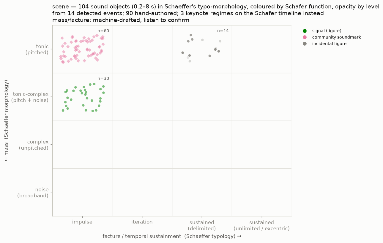
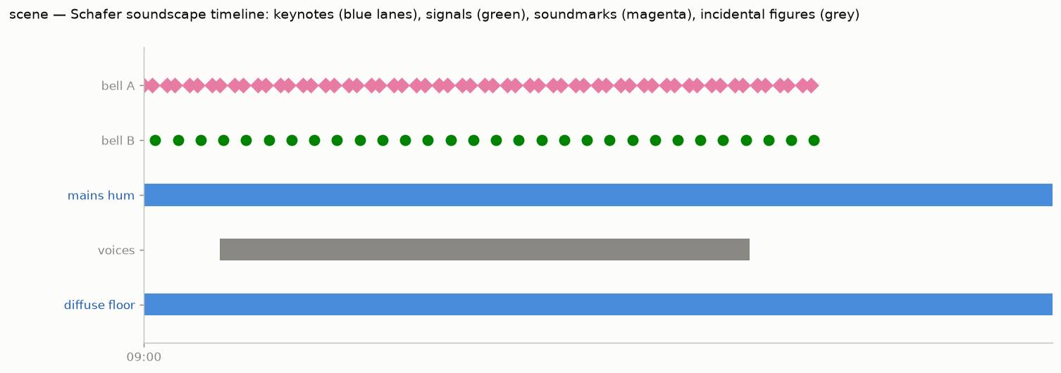
Placing a keynote regime on the typo-morphology plane therefore asks of an eight-hour ventilation bed the question Schaeffer asks of a single closing door. The two figures here keep the scales apart. The Schaeffer map is built from detected events, one point per sound object of 0.2–8 s. The Schafer timeline is built from regimes and spans, on the session clock. Neither borrows the other's unit, and the map shows no regimes at all.

Morphology without the label (objects.object_profile)

Typing an object as impulsive, sustained or iterative discards the measurements that produced the type. Two objects can share a facture and differ audibly, and a comparison — do two takes of the same action match? does a machine's onset resemble a deliberate one? — needs the numbers rather than the label.

from ambiscape.objects import object_profile
p = object_profile(env, dt)      # env: the object's amplitude envelope

field	what it says
attack_s	the 10–90 % rise towards the peak
decay_s	the fall back through a tenth of the peak, or None if the sound was cut off rather than allowed to finish
temporal_centroid	where the energy sits along the object, 0 at its start and 1 at its end
crest_db	peak over RMS
iteration_hz, iteration_strength	the envelope's best repetition rate and how strongly it repeats

The temporal centroid is the one worth knowing about. It puts impulsive and sustained on a continuous axis rather than in categories: an impulse lands near 0.04 and a held sound near 0.49, so two objects of the same facture can still be told apart.

The spectral half (objects.object_spectrum)

object_profile measures an envelope and says nothing about frequency. Pass it the object's own rows of the log-frequency spectrogram and it merges in three more, or call object_spectrum directly:

p = object_profile(env, dt, logspec=F["logspec"][i0:i1], logf=F["logf"])

field	what it says
brightness_hz	energy-weighted spectral centroid over the object
brightness_drift_oct	the last third's centroid against the first third's, in octaves — negative for an object growing duller as it decays, positive for one growing brighter
flux_per_s	frame-to-frame change of the normalised spectrum, per second, so it does not depend on the hop
n_frames	below about five, read the other three as indicative

The drift is the duration-aware one: it is a shape rather than a level, so objects of different lengths compare directly.

What they are not is a typology. Measured against listener typing on 334 labelled clips of everyday sound actions, drift runs in the predicted direction and weakly — impulsive objects at −0.25 octaves against −0.01 for iterative, p = 0.03, rank-biserial −0.16. Flux does not separate the two at all (39.5 per second against 39.7, p = 0.56) and nor does brightness. Use them to describe an object and to compare objects; use object_facture to type one.

A whole corpus of clips

ambiscape objects <folder>          # -> <folder>/objects.csv, a row per clip

Each clip is taken whole as one object and given both descriptor sets. That assumption is right for a corpus of single deliberate actions and wrong for a clip holding three events; for those, run extract_objects over a session and let the detector find the boundaries.

The cached log spectrogram has one row per second, so a six-second clip gives six and the command says how many clips fell under five rows. open_clips skips and names a file it cannot read rather than failing the batch.

These are meso-band descriptors in the sense of the timescales guide: each is defined on a single object of roughly 0.2–8 s and none needs a minute of audio. That matters for clip corpora, where the session-scale descriptors return almost nothing.

The workflow

Instruments detect when things sound. Deciding what they are, in any of the three schemes, is a listening judgement. The work is split accordingly:

ambiscape draft <folder>      # machine proposes
# ... you listen and edit ...
ambiscape taxonomy <folder>   # machine renders

1. Draft (annotations.draft.json)

From the cached features, draft pre-fills:

• steady-state keynote beds: level regimes found by change-point detection with a fixed per-regime reference (median of the regime's first two minutes) and a two-minute confirmation window, so a slammed door does not split a regime but switching off the ventilation does. The regimes are then clustered by level similarity into beds (~6 dB bands), one draft object per bed carrying all of that band's spans, named by the bed's character and extent ("quiet bed, -60 to -54 dBFS, 23 spans"); the eight longest beds are kept and any remainder is pooled into one "other beds" object. A full domestic day therefore drafts as a handful of keynote candidates rather than one object per regime. With the [ml] extra, each bed also carries a machine hint: label with the dominant PANNs tag of its longest span, explicitly marked unverified;
• detected events, each with listening hints: clock time, exceedance, level, azimuth and elevation, diffuseness, and, with the [ml] extra, AudioSet tag suggestions from PANNs. Treat those as suggestions to confirm by ear, not as ground truth.

Note that the mass and facture the draft proposes here describe regimes, and they exist only to give the annotator a starting point for the bed's character. They are not what the Schaeffer map plots: the map builds its own objects from the detected events (ambiscape.objects, described under Render below), because a regime is not a sound object.

For a third view of the same axes, in which every inter-onset segment of a short excerpt is classified on a simplified TARTYP grid, see music.tartyp_profile in Music. It needs the [music] extra.

2. Annotate (annotations.json)

The fields are grouped below by which tradition they come from. Only spans and events are ours.

Schaeffer, what the sound is in itself:

Field	Values
mass	tonic | tonic-complex | complex | noise
facture	impulse | iteration | sustained | unlimited

Schafer, what the sound does in the place:

Field	Values
kind	keynote | signal | soundmark | figure
soundmark (optional)	community | dwelling

Soundscape ecology, where the sound physically comes from:

Field	Values
source (optional)	anthrophony | biophony | geophony

Timing, ours:

Field	Values
spans / events	times as "[D ]HH:MM:SS" (D = days after day 0)

There is also an optional states list for lo-fi spans, such as a masking drone. Hi-fi and lo-fi are Schafer's terms as well: a hi-fi soundscape is one where individual sounds can be heard distinctly, and a lo-fi one is where they are crowded out.

The full schema is documented in the taxonomy module, and worked examples live in the Intercontinental database's Haarlem and Berlin session folders.

3. Render

taxonomy produces two figures, one per tradition.

The Schaeffer map: one point per sound object

The map places sound objects on the facture by mass plane, which is Schaeffer's question and his alone. Its unit is the object, not the regime: the session's detected events — the fast level rising at least 8 dB over its running background — are filtered to the object duration window (0.2–8 s by default) and each survivor is typed on both axes from its own signature in the cached features. A full domestic day yields tens of thousands of them and types in a couple of seconds, with no audio pass. Keynote regimes are counted in the caption and sent to the timeline, where they belong. The window is a choice, so it is a flag: ambiscape taxonomy <folder> --object-window 0.5 5 narrows it to Schaeffer's own figures, and the caption reports how many detected events fell outside whatever window you set.

Mass comes from the object's excess spectrum, that is, what appeared over the running band background, so a click over a ventilation drone is typed as a click and not as the drone. Two numbers are read off it, both deliberately blind to overall spectral tilt, since brightness is not mass:

• peak share, the fraction of the object's energy sitting in bands that stand 6 dB above the running median of their own octave. This is peakiness and harmonicity in one figure: a lone partial counts, every member of a harmonic series counts, and a continuum of any shape counts for nothing;
• spread, the energy-weighted standard deviation of log2 frequency, in octaves.

Reading	Mass
peak share ≥ 0.50	tonic — most of what appeared is in peaks, so a pitch is what one hears
peak share ≥ 0.20	tonic-complex — a pitch audible over a continuum that carries most of the energy
spread ≥ 1.2 octaves	noise — no pitch, energy spread wide enough to hear as a band of noise
otherwise	complex — energy in one or a few narrow regions, none of them a pitch

Facture comes from the object's own amplitude envelope, the 20 ms broadband envelope of the feature cache. Two numbers again: the attack time, the conventional 10-to-90 per cent rise towards the peak, and the iteration strength, the normalised envelope autocorrelation at its best repetition lag between 3 and 20 Hz — a single attack and decay has a monotonically falling autocorrelation and scores nothing, while a rattle, roll or grain scores at its own period.

Reading	Facture
duration ≥ 5 s	unlimited — sustainment outlasting what attention holds whole; Schaeffer's excentric case
iteration strength ≥ 0.35, duration ≥ 0.4 s	iteration — energy maintained by repetition
attack ≤ 0.08 s, duration ≤ 1 s	impulse — all the energy arrives at once and nothing maintains it
otherwise	sustained — energy held continuously between a beginning and an end

Every object carries the numbers behind both readings under _schaeffer, so any proposal can be traced back to what produced it. And they remain proposals. No public domestic corpus has object-level ground truth to score them against — activity labels are minutes long, an order of magnitude coarser than an object — so the caption keeps its "machine-drafted, listen to confirm" marking and means it.

Each object is one point, jittered inside its cell so that density is visible, with the cell's full count printed at its corner and opacity tracking the object's level, so the loud objects in a crowded cell stand out from the quiet ones. Colour is Schafer's kind — a convenience, so that you can see whether the two schemes happen to agree in your corpus — or, with activity annotations, the dominant concurrent activity. Sessions of tens of thousands of objects are subsampled for the scatter, stratified by cell so that no occupied cell disappears and stated in the caption; the printed counts always come from the full census. Hand-authored annotation entries that are themselves object-scale (events, or spans no longer than the window) join the detected ones and keep their labels where the map is sparse enough to print them.

The Schafer timeline: the keynote scale

The Schafer timeline shows the session clock, and it has two layouts; which one you get depends on whether human activity annotations are available (below). This is where the regimes live, and where they should be read: minutes and hours of ground, not objects.

The acoustic-first layout — the default, and the only one, when no activities are given — gives one lane per hand-authored object: keynote bars, signal and soundmark event markers, lo-fi states shaded, and gap-aware panels for multi-take sessions. This is where Schafer's question is answered, since a sound's function is a claim about how it sits in time and in a place. It makes statements like "the community soundmark is audible only in hi-fi windows" directly visible.

Machine-drafted steady-state regimes are the one exception to one-lane-per-object: when an annotation file still contains many of them (an unedited draft, or an older per-regime one), they are merged at render time into keynote-bed lanes by the same ~6 dB level banding the draft stage uses — at most eight bed lanes plus "other beds", each labelled with its level range and span count — so the figure height stays bounded however many regimes a long session proposes. Hand-authored objects are never merged.

Human activity ground truth (--activities)

Some datasets ship human annotations of what the people in the space were doing. The SINS database (Dekkers et al. 2017) provides per-room activity logs as semicolon-separated CSVs with a Class;Start time;Stop time header and absolute timestamps, and classes such as absence, sleeping, cooking, vacuumcleaner or watching_tv. Both figures can overlay them:

ambiscape taxonomy <folder> --activities living_labels.csv

(or taxonomy.render(folder, activities=...) / the activities parameter of schaeffer_map and schafer_timeline in the library, taking the list returned by taxonomy.load_activities). The spans are aligned to the session clock via the session's day 0; if the file is missing the figures render exactly as without the option.

The activity-first timeline

With activities present the timeline inverts, by default, into the activity-first layout: the human activities become the organising structure, not an overlay on the acoustic one. Each activity class gets a lane of its own, ordered by total time (longest first), with classes under ~0.5% of the session's labelled time pooled into an other lane at the bottom of the block. Each span's fill is coloured by its measured acoustics — the median fast level within the span, in dB re the day's median level, on the same palette as the cross-node day figures — so loud cooking and quiet cooking read differently at a glance, and a vacuum-cleaner lane lights up against a dark absence lane. Lane labels carry the acoustic summary computed from the session's cached features: "watching tv — 2.1 h, median −41 dBFS".

Hand-authored signals and soundmarks keep their own lanes and markers; the machine-drafted keynote-bed structure no longer dominates the figure but is compacted into a single strip (keynote beds — machine draft, 62 spans), its spans coloured by bed level on the same scale; the events lane stays at the foot; lo-fi states remain shaded.

Which layout applies:

• no --activities: the acoustic-first lane timeline, exactly as before;
• --activities <csv>: the activity-first layout (--layout auto, the default, or --layout activity);
• --activities <csv> --layout acoustic: the acoustic-first lane timeline with the activity material as before — a compact ribbon of coloured class spans along the top (class legend shared with the map; absence and other deliberately muted so that colour means somebody was doing something), and each machine keynote bed's label gains its dominant concurrent activities by time share: "quiet bed, -60 to -54 dBFS, 23 spans — during: absence 71%, sleeping 22%".

In the library this is schafer_timeline(..., F=..., layout=...), where F is the features dict from features.load_features; render loads the session's cached features itself when the activity-first layout needs them (without a cache the figure still renders, with neutral span fills and duration-only labels).

The map with activities

On the map, points take the colour of their dominant concurrent activity instead of their Schafer kind, with the class colours shared with the timeline ribbon's legend, and points that carry text (sparse maps, or cell-singleton outliers) also say during which activity they occur ("— during cooking"). Since every point is now one sound object, the colouring says which cells of the plane a household activity fills: dishwashing lands in impulse and noise, watching television fills the sustained column at every mass.

The two provenances are never conflated. The activities are data — human annotations shipped with the dataset, attributed in the caption (activities: human annotations, Dekkers et al. 2017) — while mass/facture, the level measurements and the bed structure remain machine output: the beds keep their "listen to confirm" marking, and the acoustic summaries are measured, not judged. Note also the scale mismatch: an activity label runs for minutes and a sound object for seconds, so the activity colour says what was going on around the object, never what the object is.

What is not here: Freesound's Broad Sound Taxonomy

A reader looking for Freesound's Broad Sound Taxonomy will not find it on this page, and the reason is the same principle the page opens with. The three schemes above each ask a question of the same sound: what it is in itself, what it does in a place, where it physically came from. The Broad Sound Taxonomy asks about the file. Is this music, an instrument sample, speech, a sound effect or a soundscape, and what would somebody use it for? That is a retrieval question, and a good one for a repository to ask, but it is not a fourth label a sound object can carry alongside the other three.

It also carries no information here. For a session recorded in a room the answer is ss-i every time, and a field with one value describes nothing. So the taxonomy lives where it is actually needed, in the upload metadata: see Deposit export.

A note on spelling

The field value is anthrophony, which is the spelling Pijanowski and most of the soundscape-ecology literature use. Both forms appear in print, and the package also accepts the older anthropophony spelling when reading an annotation file, so existing annotations keep working; everything it writes uses anthrophony.