Features and descriptors

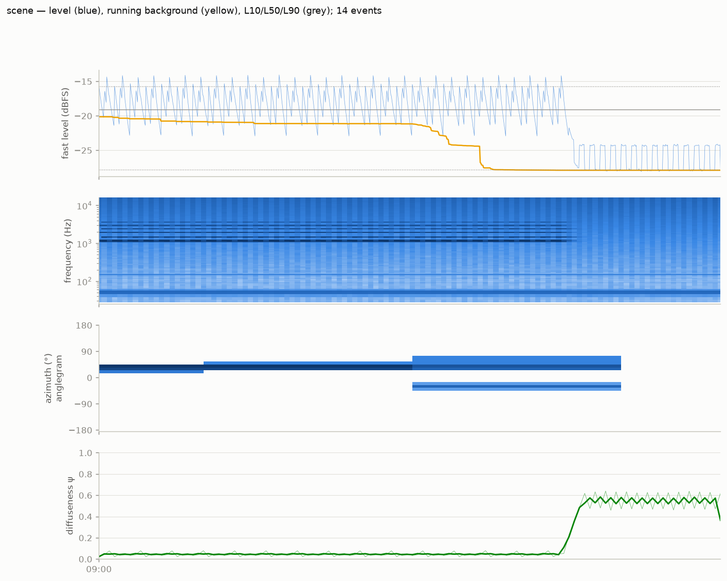
Streaming feature extraction

Files are read in 60-second blocks and never held whole in memory. Per take, cached as .npz:

Rate	Features
125 ms	fast RMS level on W, unweighted and A-weighted (IEC 61672 bilinear IIR)
1 s	octave-band powers (31.5 Hz–16 kHz), spectral centroid and flatness (50 Hz–16 kHz), 96-band log-frequency spectrogram row, per-octave pseudo-intensity vectors, broadband DOA (azimuth/elevation, 80–3000 Hz), diffuseness ψ
1 min	full-resolution (5.9 Hz bins) mean power spectrum — for narrowband hum tracking, comb/fingerprint analysis, room modes

Spectra come from Welch-style averaged 8192-point Hann FFTs at 0.1 s hops.

Spatial estimators

The pseudo-intensity vector is I(f) = Re{ W*(f) · [X, Y, Z](f) }, integrated over 80–3000 Hz (below the array's spatial-aliasing region, above wind/handling rumble). Azimuth and elevation come from its direction; diffuseness is

ψ = 1 − 2‖⟨Re W*·v⟩‖ / ⟨|W|² + ‖v‖²⟩

which is 0 for a single plane wave and 1 for an ideally diffuse field. Directional statistics over time use circular means and the resultant length R (0 = no concentration, 1 = all energy from one bearing). Foreground/background splits use energy quartiles (loudest vs quietest 25 % of seconds).

Session descriptors (summarize)

The conventions are frozen (matching the Intercontinental-database reports), so that rows stay comparable across studies:

• Leq, LAeq (energy means of the fast level), LAeq trimmed (the same A-weighted energy mean with the loudest 5 % of frames discarded, laeq_trim5_dbfs), L10/L50/L90 exceedance percentiles, dynamics L10−L90;
• events: fast level ≥ 8 dB above a running background (10th percentile in a sliding 60 s window) for ≥ 0.25 s, giving rate, count and median duration;
• spectral centroid and flatness medians;
• ψ median and IQR; energy-weighted mean azimuth and R; median foreground elevation.

Reading energy averages

Leq and LAeq are means of squared pressure, so they are decided by the loudest frames in the span rather than by the typical one. In a quiet room the distance between those two is enormous: a single slammed door can carry more energy than the hour of background it interrupts, and the average then reports the door. For scale, replacing 0.02 % of the frames of a week-long domestic recording with full-scale material—sixteen frames in ninety-odd thousand—moves that week's LAeq by more than 4 dB and its Leq by nearly 3 dB, while L10, L50, L90, the dynamics L10−L90 and the trimmed LAeq stay bit-identical. Nothing about that arithmetic is peculiar to artefacts; a handful of genuine loud events does the same thing, which is why an energy average alone cannot be read as a description of a quiet space.

Practical consequences:

• Never quote LAeq on its own. Report it beside the trimmed level (laeq_trim5_dbfs) or a percentile. Agreement between the two says the average describes the span; a large gap says it describes a few moments, and both numbers are then worth printing.
• In quiet rooms, lead with the percentiles. L50 and L90 and the dynamic range L10−L90 are the primary descriptors of a background, with LAeq as the supporting energy figure. Comparisons between periods, rooms or nodes are stable on percentiles and fragile on energy means, which can differ by several decibels for reasons that have nothing to do with the quality being compared.
• Descriptors built on LAeq inherit the fragility. Emergence (LAeq − LA90) and any level-based day/night or state contrast move with the loudest frames; the trimmed level gives the same contrast without them.
• Percentile levels have their own failure mode. A low percentile can measure the recorder rather than the room—see the sensor-noise-floor guard below and the floor_suspect flag in summary.json before trusting L90 in a quiet high-band scene.

Reading ψ and R together

High ψ + high R = diffuse but anisotropic (an airport hall that "leans" one way). Low ψ + high R = a point-source room (one running machine). Low R with any ψ = scattered sources.

Spectral foreground (per-band background)

background.band_background runs a low-percentile filter per log band (default: 10th percentile over 300 s), from the cached 1 Hz logspec, with no audio pass. On top of it:

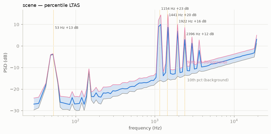
• foreground fraction—the share of total power sitting > 3 dB above the spectral background, per second (steady scenes score low even when loud; transient-dominated scenes score high even when quiet);
• spectral events—connected time × band regions of ≥ 6 dB exceedance: band-limited events (a distant bell over traffic, a bird band, a beep) that the broadband ±8 dB detector never sees. Each carries onset, duration, band span, and peak rise.

analyze appends fg_fraction_median, fg_fraction_p90, spectral_events_per_min, and spectral_event_median_dur_s to the summary.

Sensor-noise-floor guard

A low-percentile level can measure the recorder rather than the room. In the SINS sensor-network corpus the 4–8 kHz background floor of a living room is flat to 0.8 dB across a full week (0.56 dB between six separate nights), while every band below 1 kHz varies by 2.4–5.3 dB over the same nights: the top of the spectrum is microphone self-noise, and A-weighting emphasises exactly that region, so LA90 there measures the recorder.

analysis.floor_suspicion (run as part of every summarize) checks each octave band centred at 2 kHz and above: the session is cut into 300 s chunks, each chunk's 10th-percentile band level is its floor, and the temporal spread is taken as the median minus the 5th-percentile chunk floor — a low-tail statistic, so chunks whose floor is raised by activity do not hide a pinned quiet-time floor. A spread under 1.5 dB flags the band: the threshold sits between the SINS self-noise band (≤ 0.8 dB) and the quietest genuinely acoustic bands there (≥ 2.4 dB), with at least 0.7 dB of margin to each side. summary.json gains floor_suspect (boolean), the affected band range floor_suspect_lo_hz / floor_suspect_hi_hz, and floor_spread_db; when the flag fires, the session README carries a warning that L90-derived descriptors in that range may reflect the recorder, not the room.

This is an annotation, not a correction — no descriptor value changes. Sessions shorter than six chunks (30 min) are never flagged, and bands with no content below the Nyquist frequency are excluded.

How much of the session is floor (floor_occupancy, 0.29.0)

The guard above asks whether a band's floor is self-noise. Run across a whole sensor network it tends to fire for every node, because every recorder's top octaves are its own hiss during quiet hours — so it cannot separate "this band is the recorder" from "this room was empty all week".

analysis.floor_occupancy asks the second question: what fraction of the session sits within a few dB of that session's own floor. Across the SINS network the living-room and kitchen nodes read 0.28–0.56 while the bedroom node reads 0.96, a median of 0.4 dB above its own floor against 2.4–9.8 dB for rooms in use.

That is a description of how a room is used, not a fault in the recorder — a distinction worth having, since a microphone in a mostly-empty bedroom otherwise looks exactly like a broken one. Being each session against its own floor, the measure does not move with recording gain, so it compares across uncalibrated instruments where an absolute level cannot.

Which capsule to read (quietest_channel, 0.30.0)

A multi-microphone node's capsules share a housing, a preamp and a gain setting, so they should agree. When one does not — a blocked port, a damaged capsule — it reaches the same peaks as its siblings on a raised floor, and so has less room to measure in. Reading channel 0 by convention is then a coin toss.

analysis.quietest_channel(x, fs) returns the channel with the lowest floor and every channel's floor, so the caller can see whether the choice matters. In the SINS network one node's four capsules reached the same 98th-percentile level within 0.7 dB while channel 0's floor sat 5.5 dB higher: analysing channel 0 halved that node's apparent dynamics and pushed its time-at-own- floor from about 75 % to 96 %. On nodes whose capsules agree, the function picks whichever is marginally lower, which is of no consequence.

Modulation profile (modspec)

Environmental rhythm at three scales from cached envelopes: micro (0.5–20 Hz strike/speech-rate rhythm, from the 20 ms env_hi envelope), meso (0.01–0.5 Hz: traffic waves, surf), macro (duty cycles below 0.01 Hz). Per scale: a log-frequency modulation spectrum, the dominant modulation frequency and its prominence, and a band modulation depth; plus a windowed "rhythm spectrogram" of the session. Caches from extractor versions without env_hi fall back to the 8 Hz fast level (micro < 4 Hz).

Tonality and harmonicity (tonality)

From the per-minute mean PSD: prominent narrowband peaks are linked into tonal tracks (hums, bell partials and beeps, with duration and cents drift); a harmonic sieve finds the best f0 per minute and scores harmonicity (bells score low, since their partial series is not harmonic); tonal energy folds onto a 12-bin pitch-class profile ("what key does the soundscape hum in").

Spatial dynamics (spatial)

Per-octave directness (|pseudo-intensity| / band power, the spatial analogue of foreground/background), pass-by detection (level events whose azimuth sweeps monotonically: moving sources with rate and direction), and the azimuth organisation timeline R(t), which is the windowed, energy-weighted circular concentration of the direction of arrival.

Schedule matching (schedule)

Folds event streams at civic periods (minute, 5-min, quarter, half-hour, hour, day) and scores each with circular statistics. Read n_cycles before trusting a match: R is trivially 1 when all events fall inside one grid cycle. schedule.clock_offset turns an event of known wall-clock time into the clock_offset_s calibration value.

Event timbre templates (timbre)

Each spectral event gets a fingerprint—mel-band rise spectrum (what appeared) plus per-band decay slope (how it faded)—and fingerprints are clustered by correlation into recurring event classes: "the same sound again" across a session, transparent and corpus-comparable, no ML.

Masking (background.masking_index)

Floor elevation per band between a source-active and a quiet state: how much a dominant source hides the rest of the field, and in which bands. Often frequency-selective, as when the Haarlem bells elevate the typical floor 9–14 dB in their partial bands while the rest of the spectrum stays nearly free.

MIR views (music, optional)

With pip install "ambiscape[music]", ambiscape music renders the MIR-standard tempogram (onset autocorrelation in BPM, with librosa's octave-resolved global tempo) and chromagram, which cross-check the built-in windowed-ACF tempogram and pitch-class profile.

Segment selection

pick_segments proposes representative windows for listening, archiving, ISO indicators, or ambiviz rendering: the quietest, the most active, the typical, and (when a >6 dB state change exists) the transition.