Environmental rhythm (modulation profile)

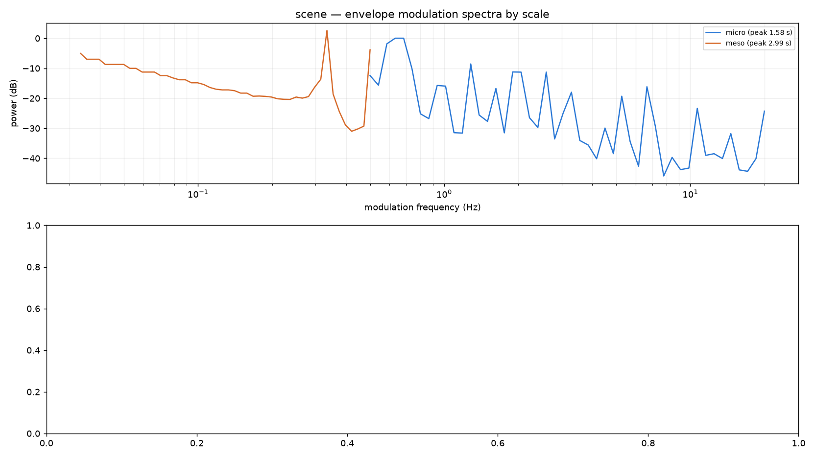
A soundscape is rhythmic on very different time scales at once: bell strikes and footsteps beat at a few hertz, traffic waves and surf breathe over tens of seconds, and machines and human activity switch on a duty cycle of minutes to hours. ambiscape modspec measures all three from the cached envelopes — no second pass over audio — as a modulation profile: a log-frequency modulation spectrum per scale, plus a rhythm spectrogram of the whole session.

ambiscape modspec <session-folder>   # needs a prior analyze run

Writes modulation.json (per-scale dominant modulation frequency, period, prominence and band modulation depth, plus the raw spectra) and modulation_profile.png (the spectra by scale over a 10-minute-window rhythm spectrogram, in dB relative to each window's median).

The three scales

• micro (0.5–20 Hz) from the 20 ms broadband envelope — strike patterns, footstep cadence, flutter. This needs the high-rate env_hi cache (extractor ≥ 0.2); on older caches micro falls back to the fast level and tops out at 4 Hz (flagged as micro_limited in the JSON).
• meso (0.01–0.5 Hz) from the 125 ms fast level — traffic waves, surf, wind gusts, conversational turn-taking.
• macro (below 0.01 Hz, floor set by session length) from the 1 s RMS — ventilation and appliance duty cycles, diel activity.

Each scale reports peak_freq_hz, peak_period_s, peak_prominence_db (peak over the band median) and modulation_depth (band-integrated modulation power of the unit-mean envelope). A sharp, prominent peak means periodic structure; a flat spectrum means the level just wanders.

In Python

from ambiscape import modulation

prof = modulation.profile(F)          # F = load_features(...)
prof["scales"]["meso"]
# {'peak_freq_hz': 0.033, 'peak_period_s': 30.0,
#  'peak_prominence_db': 7.4, 'modulation_depth': 0.21}

modulation.modulation_spectrogram(env, dt) returns the windowed version directly — (t_centers, mod_freqs, S) — if you want to build the rhythm spectrogram from a custom envelope.