Spaced-microphone array

The toolbox reads space in three ways, differing in where the microphones sit. Spatial analysis reads a soundfield sampled at one point — co-located ambisonic capsules — and asks from which direction; the multi-room acoustic network reads one microphone per room and asks through which fabric; array sits between them: a handful of spaced omnis in one room, the SINS nodes' linear four-MEMS arrays being the model case. Across a spaced array a wavefront arrives at each capsule at a slightly different time, and the pattern of those arrival-time differences carries a bearing; how coherent the channels remain across frequency carries a direct-versus-diffuse reading. Neither needs a soundfield microphone to have been present.

ambiscape array node.wav --geometry geometry.json
#   4 mics, 6 pairs, 1199 frames of 0.100 s
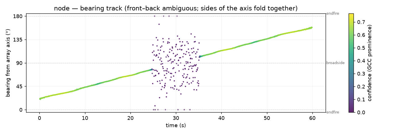
#   bearing median 62.1° from the axis (IQR 4.0°), confident frames 81% — front-back ambiguous, endfire-blind
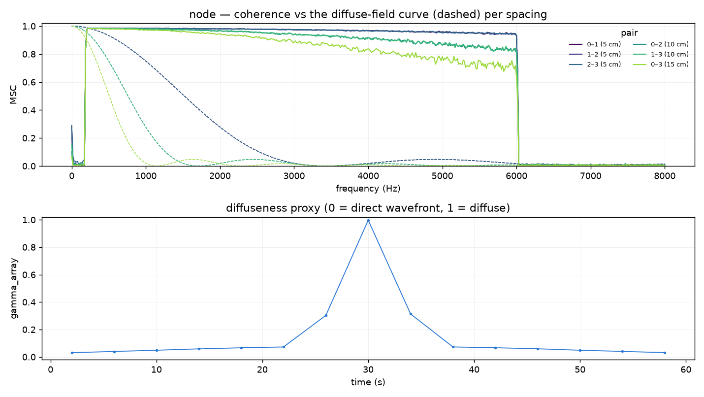
#   gamma_array median 0.24 (0 = direct wavefront, 1 = diffuse; spaced-omni proxy, not the FOA psi)
#   wrote analysis/array.json and 2 figure(s)

ambiscape array node.wav --spacing 0.05      # uniform linear shortcut

The geometry file gives mic positions in metres (and optionally the speed of sound); a flat list is read as positions along one line:

{"mics": [[0.0, 0.0], [0.05, 0.0], [0.10, 0.0], [0.15, 0.0]], "c": 343.0}

How it works

• TDOA (tdoa) — every frame (default 100 ms, hopped by half) is Hann-windowed and, per mic pair, the PHAT-weighted cross-power spectrum is inverted to a generalised cross-correlation (GCC-PHAT). The peak is searched only over physically possible lags (± spacing / c) and refined by parabolic interpolation. Convention: tau_s[frame, pair] = t_i − t_j for pair (i, j), positive when the wavefront reaches mic j first. Each estimate carries the GCC peak height (1 for a clean single delay, near 0 for decorrelated channels) and its prominence over the strongest rival lag — the confidence base.
• Bearing (bearing) — for mics on one line with axis u, a plane wave from cone angle θ gives tau_ij = −(s_i − s_j) cos θ / c, so each frame's cos θ is a prominence-weighted least-squares fit across all pairs. Bearings run 0–180° from the axis (0/180 = endfire, 90 = broadside); the confidence stream is the median GCC prominence across pairs, and frames whose fit falls outside |cos θ| ≤ 1 are flagged clipped.
• Coherence profile (coherence_profile) — per window (default 4 s) the magnitude-squared coherence of every pair versus frequency, next to the analytic diffuse-field curve for spaced omnis at that spacing, sinc(2 f d / c)².
• Diffuseness proxy (gamma_array) — per window, the energy-weighted excess of measured coherence over the diffuse curve (taken where the curve has fallen below 0.5, so the spacing is informative) is normalised to a directness reading; gamma_array is one minus its median across pairs: 0 when a coherent wavefront crosses the array, 1 when coherence sits at or below the diffuse prediction.

Honest limits

• Front–back ambiguity — a linear array observes only the cone angle: the two sides of its axis fold onto one bearing, and nothing in the data can unfold them. Triangulation resolves the fold only when the node geometry breaks the mirror symmetry (see below).
• Endfire blindness — near 0° and 180° the delay–angle mapping flattens (dτ/dθ → 0), so endfire bearings are low-resolution even at high confidence, and fits pushed past the physical limit are clipped to the endfire and flagged.
• gamma_array is a proxy — it is built from spaced-omni coherence deviations and is deliberately named apart from the first-order-ambisonic diffuseness ψ (diffuse in the feature cache), an energetic soundfield measure at a single point. The two agree in tendency, not in value; do not pool them in one column.
• One clock per node — TDOAs compare channels of one interface, so sample-synchronous capture is assumed within a node. Across nodes only bearings are combined, never sample times.

What it produces

• array.json — geometry, per-pair median TDOAs (ms), bearing summary over the confident frames (median, IQR, confident fraction), and the gamma_array median and IQR.
• array_bearing.png — the bearing track, time × bearing with the confidence as colour (linear geometries only).
• array_coherence.png — measured coherence per spacing against the dashed diffuse-field curves, over the gamma_array timeline.

Triangulation across nodes

With two or more nodes bearing on the same event, triangulate intersects the bearing streams on a floor plan by weighted least squares — a library call, since it needs several recordings on a shared clock. The floor plan gives each node's position and the world direction of its array axis (anticlockwise from +x, first mic towards last):

{"nodes": [
  {"name": "living",  "pos": [0.0, 0.0], "axis_deg": 0.0},
  {"name": "kitchen", "pos": [4.0, 0.0], "axis_deg": 90.0}
]}

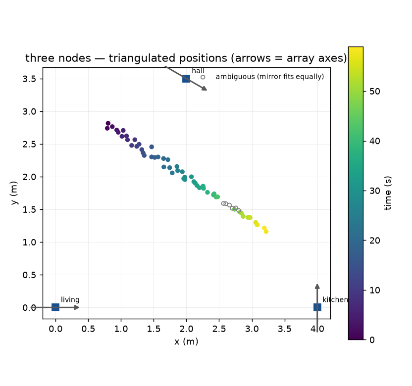
Each linear-array bearing admits two world rays, axis_deg ± bearing; every sign combination is solved and the one with the smallest residual wins, with rays that would place the source behind a node rejected. When the runner-up fits almost as well — parallel array axes make the two sides genuinely indistinguishable — the fix is flagged ambiguous rather than silently resolved. With exactly two nodes any two non-parallel rays meet exactly, so only mirror rays that fall behind a node can be eliminated; a third node makes the residual itself discriminating. The residual (RMS ray-to-point distance) is the coarse uncertainty: treat each position as a blob of about that radius, and distrust fixes whose intersection angle is small.

A worked synthetic example, with the bearing streams built directly from the plan geometry (in practice they come from bearing(tdoa(...)) per node):

import numpy as np
from ambiscape import array

plan = {"nodes": [
    {"name": "living",  "pos": [0.0, 0.0], "axis_deg": 0.0},
    {"name": "kitchen", "pos": [4.0, 0.0], "axis_deg": 90.0},
]}

def stream(pos, axis_deg, source, n=60):
    """The bearing a node at ``pos`` would report for ``source``."""
    v = np.subtract(source, pos)
    world = np.degrees(np.arctan2(v[1], v[0]))
    theta = abs((world - axis_deg + 180) % 360 - 180)   # cone angle
    return {"t": np.arange(n, dtype=float),
            "bearing_deg": np.full(n, theta),
            "confidence": np.full(n, 0.8),
            "clipped": np.zeros(n, bool)}

source = (1.5, 2.0)
tri = array.triangulate([stream((0, 0), 0.0, source),
                         stream((4, 0), 90.0, source)], plan)
tri["xy"][0]                                  # -> [1.5, 2.0]
array.triangulate_figure(tri, plan, "triangulation.png")

When the spacing was never written down

Everything above needs load_geometry — the mic positions in metres. Plenty of archives do not have them. near_source_index is the fallback: mean inter-channel coherence in one band, averaged over every channel pair, assuming nothing about which channel sits where.

from ambiscape.array import near_source_index
v = near_source_index(x, fs, band=(500.0, 1000.0))   # x is (samples, channels)

It answers one question — how directional is this moment — and it answers it without calibration, because a ratio between two channels of one device divides that device's gain out. On a network of uncalibrated nodes that is worth a good deal: on the SINS corpus a single fixed threshold, no per-node tuning, separates loud activity from an empty room at 95.5 % across twelve nodes.

It is not an occupancy detector. Over 749 labelled minutes of that corpus a television playing to an empty room scored higher than any class with a person in it (0.717 against 0.678 for a vacuum cleaner), and a person working quietly scored 0.365 against 0.247 for an empty room. It detects a near sound source. A loudspeaker is one; a silent person is not.

Two practical points. Keep band below the array's spatial aliasing limit, c / 2d — under about 2 kHz is safe for capsules a few centimetres apart, and a band that is too high collapses towards zero for every input alike. And the reading is comparable only against itself and against arrays of the same build: there is no absolute scale, which is the price of taking no geometry.

Programmatic helpers

ambiscape.array exposes the pieces directly: load_geometry, tdoa, bearing, bearing_figure, near_source_index, coherence_profile, coherence_figure, load_plan, triangulate, triangulate_figure, and run_array. See the API reference.