This week we turn to psychoacoustics, the study of how we perceive and interpret sound. In terms of the four levels of description, we now move from the physical and electronic signals we have explored during the past two weeks to perception. There are many similarities between machine and human perception, but there are also some important differences: equal-loudness contours, masking, and the missing fundamental are examples of where the ear reports something the microphone does not. Why does one sound seem louder than another of the same intensity? How do we tell a violin from a piano playing the same note, and why do some sounds please us while others grate? Questions like these set up the more detailed look at “vertical” and “horizontal” sound perception in the coming weeks.
Introduction to psychoacoustics
Psychoacoustics is a branch of psychophysics, the study of how physical stimuli relate to the sensations and perceptions they produce. Psychophysics covers all the senses; psychoacoustics narrows the focus to hearing. Both use experiments to measure how changes in physical properties such as frequency, intensity, or duration map onto changes in perception such as pitch, loudness, or timbre.
These insights have practical uses. They inform audio engineering, music production, and hearing aid design, and they underpin audio codecs such as MP3 and AAC, which exploit the limits of perception to compress audio without an audible loss in quality.
The roots of the field of psychoacoustics go back to the 19th century. Hermann von Helmholtz (1821–1894) studied the sensations of tone and the physical basis of music, and later S. S. Stevens (1906–1973) developed methods for psychophysical scaling that quantify the relationship between a stimulus and how it is perceived. Since then the field has grown to draw on physics, psychology, neuroscience, and engineering.
Auditory perception covers the processes by which the ear and brain detect, analyse, and make sense of acoustic signals, turning vibrations in the air into speech, music, or environmental sounds. Psychoacoustics explains the perceptual side of this: why a sound is heard as louder, higher, or more pleasant, and how we separate different sources in a complex scene.
Cognition adds the higher-level functions: attention, memory, learning, and decision-making. Where psychoacoustics deals with the sensory and perceptual mechanics of hearing, cognition shapes how we interpret, remember, and respond to what we hear. Cognitive processes let us follow a single voice in a noisy room (the “cocktail party effect”), recognise a familiar melody, or tie a sound to an emotion or memory. We will explore several of these topics in the coming weeks.
The human auditory system
The human ear lets us detect sounds and keep our sense of balance. It has three main sections: the outer ear, middle ear, and inner ear, each with a distinct job in the hearing process.
The outer ear
The outer ear consists of the visible part called the pinna and the ear canal. Its job is to collect sound waves from the environment and funnel them towards the eardrum (sometimes called the tympanic membrane). The shape of the pinna helps us locate the direction a sound comes from. When sound waves reach the eardrum, they make it vibrate.
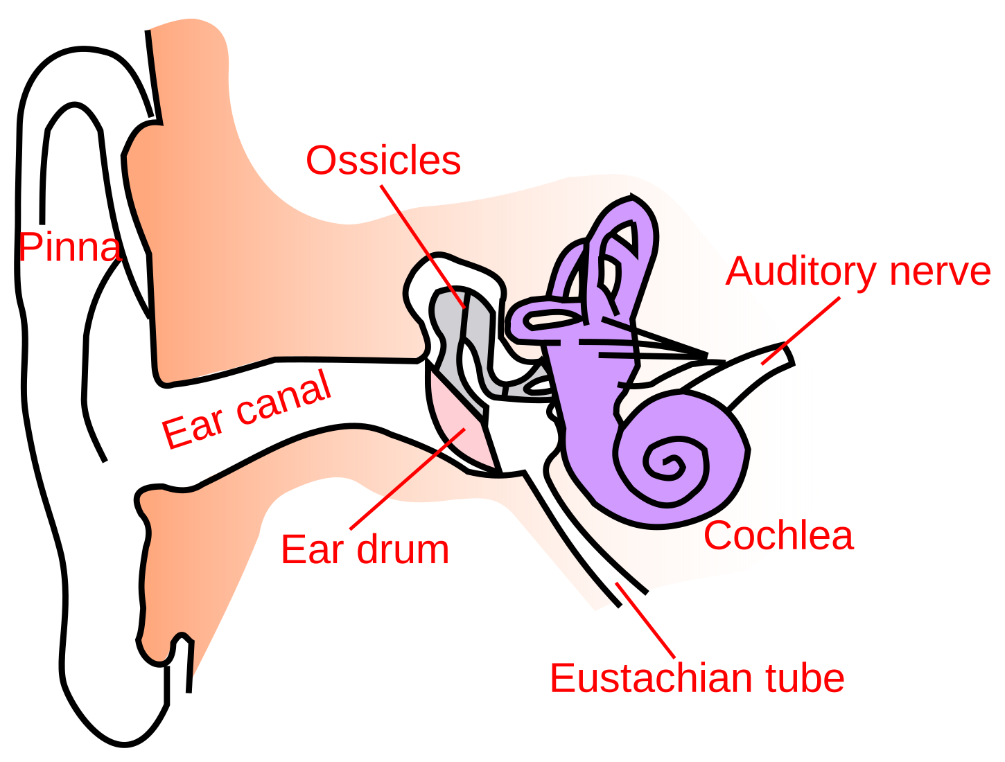
Image Source: Wikipedia - Outer Ear
The eardrum works much like the membrane in a microphone, familiar from the previous chapter. Both are sensitive barriers that vibrate in response to incoming sound waves. In the ear, vibrations of the eardrum pass through the ossicles to the inner ear, where they become electrical signals for the brain to interpret. In a microphone, sound waves hit a thin, flexible diaphragm; its vibrations are converted into electrical signals that can be amplified, recorded, or transmitted. In both cases, air pressure variations become mechanical vibrations, which is the first step in turning acoustic energy into a form that can be processed further, biologically in the ear and electronically in the microphone.
The middle ear
Beyond the eardrum lies the middle ear, which contains three tiny bones known as the ossicles: the malleus, incus, and stapes. These bones act as a mechanical lever system, amplifying the vibrations from the eardrum and passing them to the oval window, a membrane-covered opening to the inner ear. The amplification helps sound energy transfer efficiently from air into the fluid-filled inner ear.
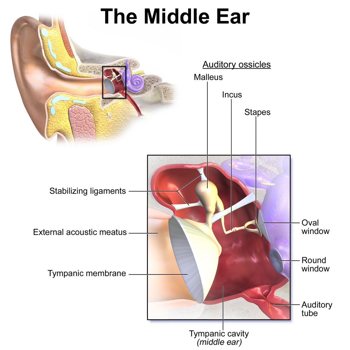
Image Source: Wikipedia - Middle Ear
The amplification in the ear resembles how a signal from a microphone membrane is sent through a preamplifier to bring it up to a level suitable for recording or further processing. In the same way, the ossicles boost the mechanical vibrations from the eardrum so the signal is strong enough to drive the inner ear.
The inner ear
The inner ear is where mechanical vibrations become electrical signals that the brain can interpret as sound. The main structure for this is the cochlea, a spiral-shaped, fluid-filled organ lined with thousands of tiny hair cells. As vibrations travel through the cochlear fluid, they move the hair cells, generating nerve impulses that travel to the brain along the auditory nerve.
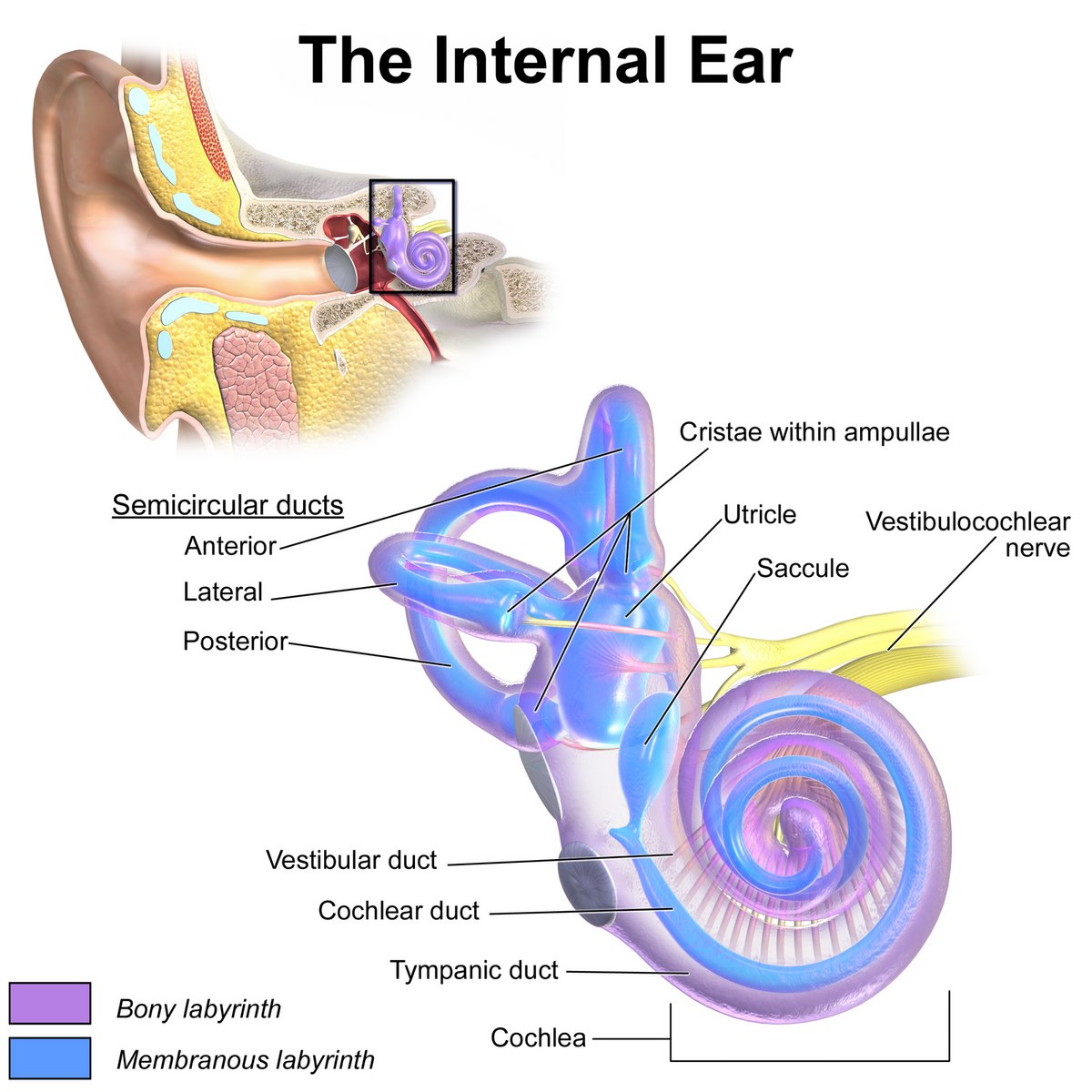
Image Source: Wikipedia - Inner Ear
The hair cells are laid out in an orderly map. Those near the base of the cochlea respond best to high frequencies, those near the apex to low ones. This frequency map is called tonotopic organisation, or tonotopy,, and it is preserved all the way up to the auditory cortex (see the brain). It means the ear delivers something close to a spectrum to the brain, rather than a raw waveform.
The cochlea works rather like the analogue-to-digital converter (ADC) from the previous chapter. An ADC turns continuous analogue sound waves into discrete digital signals that a computer can process; the cochlea turns mechanical vibrations into electrical nerve impulses that the brain can read. Inside the cochlea, different hair cells respond to different frequencies, so the organ performs a biological frequency analysis while also encoding the intensity and timing of sounds, much as an ADC samples and quantises an audio signal.
The inner ear also contains the vestibular system, which keeps us balanced and spatially oriented. We will return to this when we get to music-related body motion.
Human vs machine perception
The human auditory system and machine-based audio systems are built on completely different biological and technological foundations, but the analogy between them is useful. Each is a chain of components that transforms and processes sound, turning physical vibrations in the air into meaningful information: neural signals in the brain, digital data in a computer.
Even though there are some similarities between the two, there are also important differences:
- The human auditory system is adaptive and context-sensitive, shaped by attention, learning, and memory. It can pick out specific sounds in noisy surroundings (the “cocktail party effect”) and fill in missing information from prior experience.
- Machine perception is bounded by hardware (microphone quality, sampling rate) and by the algorithms used for analysis. Modern systems can do impressive work, but they lack the flexibility and subjective interpretation of human hearing.
These parallels and differences matter for audio engineering, hearing aid design, and music information retrieval, where the aim is often to connect physical sound with perceptual experience.
Loudness
As we saw in the acoustics chapter, loudness is not the same as sound pressure level (SPL). The latter is an objective, physical measurement of the intensity of a sound wave, expressed in decibels (dB). Loudness is the subjective side: how “loud” a sound feels to a listener. It is shaped by context, such as background noise and recent exposure to other sounds, and the gap between the two runs through much of audio engineering, hearing science, and music production.
Measuring loudness
The most common unit for perceived loudness is the phon, which is based on equal-loudness contours (more on these below). The phon scale is anchored to a 1,000 Hz pure tone. A sound judged as loud as a 40 dB SPL, 1,000 Hz tone has a loudness of 40 phons, whatever its own frequency or SPL. The phon says which sounds are equally loud, not how much louder one is than another. For that there is the sone: 1 sone is defined as 40 phons, and each doubling of perceived loudness adds one more sone, so a sound of 4 sones is heard as twice as loud as one of 2 sones. Roughly, every 10 phons doubles the number of sones.
Modern audio software and digital audio workstations (DAWs) often include loudness meters that display values in LUFS: loudness units relative to full scale. These tools help engineers and producers meet broadcast standards and keep listening comfortable.
Dig deeper: loudness standards
Several standards exist for estimating loudness in audio signals, and they serve two different purposes.
The first group measures programme loudness so that broadcasts and streams can be normalised. ITU-R BS.1770 is the foundation: it defines the K-weighted measurement behind LUFS, the gating that ignores silence, and the true-peak level. Regional recommendations build on it. EBU R 128 in Europe sets a target of −23 LUFS and adds the loudness range measure and the momentary and short-term meters that DAWs display, while ATSC A/85 in the United States sets −24 LKFS and underpins the CALM Act, which stopped television commercials being louder than the programmes around them. Streaming platforms use the same measurement with their own targets: Spotify and YouTube normalise to about −14 LUFS and Apple Music to −16 LUFS. These are platform practices rather than formal standards, but they are the numbers you meet when mastering.
The second group models perceived loudness itself. ISO 532 specifies two psychoacoustic loudness models, the Zwicker method and the Moore–Glasberg method, which compute loudness in sones from a sound’s spectrum, taking masking between frequency bands into account. ISO 226 defines the standard equal-loudness contours, the modern successor to the Fletcher–Munson curves shown below, and is what the phon scale is anchored to today.
Equal-loudness contours
SPL and loudness are related but not the same. The same SPL can be heard as louder or softer depending on the frequency of the sound and the listener’s hearing sensitivity.
Harvey Fletcher and Wilden A. Munson studied this systematically in the 1930s. Their experiments Fletcher & Munson, 1933 produced the Fletcher–Munson curves, now usually called equal-loudness contours. The curves show that the ear is not equally sensitive across frequencies. We hear best between roughly 2,000 and 5,000 Hz, and are less sensitive to very low or very high frequencies. So a low-frequency sound has to be played at a higher SPL than a mid-frequency sound to seem equally loud.
The figure below shows the contours as standardised today in ISO 226, from the threshold of hearing up to 80 phons. Each curve joins the sound pressure levels at which pure tones of different frequencies sound equally loud, and at 1,000 Hz the phon value equals the level in dB SPL.
Source
import numpy as np
import matplotlib.pyplot as plt
plt.rcParams.update({
    "font.size": 10,
    "axes.titlesize": 11,
    "axes.labelsize": 10,
    "xtick.labelsize": 9,
    "ytick.labelsize": 9,
    "legend.fontsize": 9,
    "figure.figsize": (10, 4),
    "figure.dpi": 100,
    "savefig.dpi": 150,
    "axes.spines.top": False,
    "axes.spines.right": False,
})

# Equal-loudness contours from ISO 226:2003 (valid from 20 to 90 phons, 20 Hz to 12.5 kHz)
f = np.array([20, 25, 31.5, 40, 50, 63, 80, 100, 125, 160, 200, 250, 315, 400, 500, 630, 800,
              1000, 1250, 1600, 2000, 2500, 3150, 4000, 5000, 6300, 8000, 10000, 12500])
af = np.array([0.532, 0.506, 0.480, 0.455, 0.432, 0.409, 0.387, 0.367, 0.349, 0.330, 0.315, 0.301,
               0.288, 0.276, 0.267, 0.259, 0.253, 0.250, 0.246, 0.244, 0.243, 0.243, 0.243, 0.242,
               0.242, 0.245, 0.254, 0.271, 0.301])
Lu = np.array([-31.6, -27.2, -23.0, -19.1, -15.9, -13.0, -10.3, -8.1, -6.2, -4.5, -3.1, -2.0, -1.1,
               -0.4, 0.0, 0.3, 0.5, 0.0, -2.7, -4.1, -1.0, 1.7, 2.5, 1.2, -2.1, -7.1, -11.2, -10.7, -3.1])
Tf = np.array([78.5, 68.7, 59.5, 51.1, 44.0, 37.5, 31.5, 26.5, 22.1, 17.9, 14.4, 11.4, 8.6, 6.2, 4.4,
               3.0, 2.2, 2.4, 3.5, 1.7, -1.3, -4.2, -6.0, -5.4, -1.5, 6.0, 12.6, 13.9, 12.3])

def contour(phons):
    """Sound pressure level (dB SPL) of a pure tone at each frequency that is heard as `phons` loud."""
    Af = 4.47e-3 * (10 ** (0.025 * phons) - 1.15) + (0.4 * 10 ** ((Tf + Lu) / 10 - 9)) ** af
    return (10 / af) * np.log10(Af) - Lu + 94

levels = [20, 40, 60, 80]
blues = plt.cm.Blues(np.linspace(0.45, 0.95, len(levels)))

fig, ax = plt.subplots(figsize=(10, 5))
ax.semilogx(f, Tf, color='grey', linestyle='--', linewidth=1.5)
ax.text(13500, Tf[-1], 'threshold\nof hearing', color='grey', va='center')
for phons, color in zip(levels, blues):
    L = contour(phons)
    ax.semilogx(f, L, color=color, linewidth=2)
    ax.text(13500, L[-1], f'{phons} phons', color=color, va='center')
ax.axvline(1000, color='grey', linestyle=':', linewidth=1)
ax.text(950, 108, 'at 1,000 Hz, phons = dB SPL', ha='right', color='0.3')
ax.axvspan(2000, 5000, color='0.93', zorder=0)
ax.text(3150, 100, 'most\nsensitive', ha='center', color='0.3')
ax.set_xlim(20, 20000)
ax.set_ylim(-10, 115)
ax.set_xticks([20, 50, 100, 200, 500, 1000, 2000, 5000, 10000])
ax.set_xticklabels(['20', '50', '100', '200', '500', '1k', '2k', '5k', '10k'])
ax.set_xlabel('Frequency (Hz)')
ax.set_ylabel('Sound pressure level (dB SPL)')
ax.set_title('Equal-loudness contours (ISO 226:2003)')
ax.grid(True, which='both', alpha=0.3)
plt.tight_layout()
plt.show()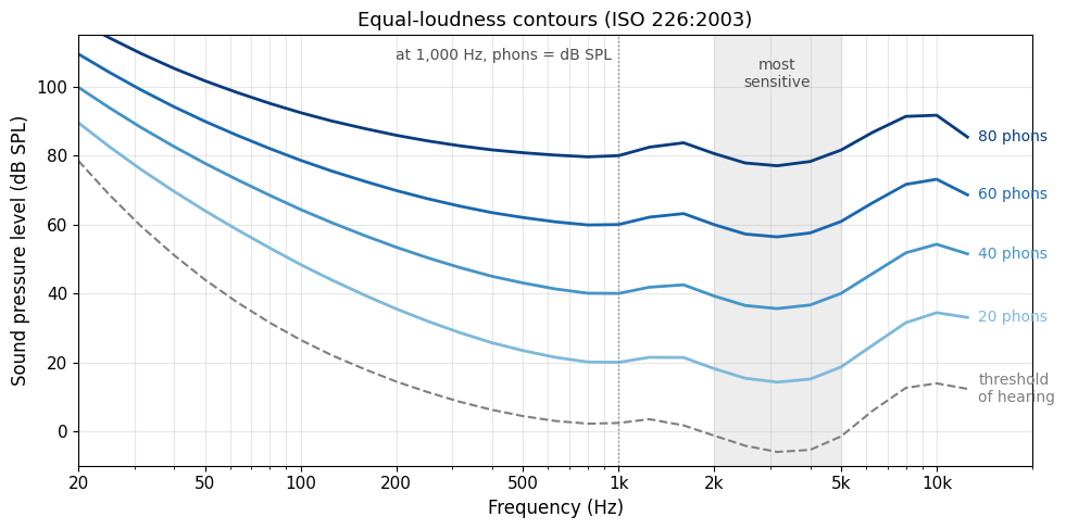
Our heightened sensitivity between 2,000 and 5,000 Hz may have evolutionary roots. This range matches the spectral content of human speech, especially the consonants that carry much of the meaning. Picking up small differences in these frequencies would have helped with communication and with detecting important sounds such as a baby’s cry or a warning call. Over time, natural selection may have favoured hearing tuned to this range.
Equal-loudness contours matter in audio engineering, music production, and hearing science. They explain why music or speech sounds different at low and high volumes, and why audio equipment often includes a “loudness” control that compensates for these perceptual differences.
Threshold of hearing
The threshold of hearing is the quietest sound the average ear can detect in a silent environment. It is usually defined as 0 decibels (dB SPL) at 1,000 Hz for a healthy young adult, but it varies with frequency and with individual hearing. At very low or very high frequencies, a sound has to be much louder before we hear it.
The threshold is not fixed. It shifts with age, with exposure to loud noise, and even with temporary conditions such as an ear infection or fatigue. As people age, sensitivity to high frequencies usually drops, raising the threshold there.
The absolute threshold is the lowest curve in the equal-loudness figure above: the sound pressure level a pure tone needs before a young adult with normal hearing detects it at all. The figure below shows what age does to it, in the form of typical audiograms for three ages. An audiogram plots the threshold relative to normal young hearing (dB HL, hearing level), with worse hearing further down the chart, and shows how the loss with age concentrates at the high frequencies.
Source
import numpy as np
import matplotlib.pyplot as plt
plt.rcParams.update({
    "font.size": 10,
    "axes.titlesize": 11,
    "axes.labelsize": 10,
    "xtick.labelsize": 9,
    "ytick.labelsize": 9,
    "legend.fontsize": 9,
    "figure.figsize": (10, 4),
    "figure.dpi": 100,
    "savefig.dpi": 150,
    "axes.spines.top": False,
    "axes.spines.right": False,
})

# Typical audiograms (dB HL) by age, approximate median values after ISO 7029
f_aud = np.array([125, 250, 500, 1000, 2000, 4000, 8000])
ages = {'20 years': [2, 2, 2, 2, 2, 3, 5],
        '40 years': [4, 4, 4, 5, 7, 11, 17],
        '60 years': [7, 8, 9, 10, 15, 27, 40]}
colors = ['steelblue', 'darkorange', 'firebrick']

fig, ax = plt.subplots(figsize=(10, 4.5))
for (label, vals), color in zip(ages.items(), colors):
    ax.semilogx(f_aud, vals, 'o-', color=color, linewidth=2, markersize=6, label=label)
ax.axhspan(-10, 20, color='0.92', zorder=0)
ax.text(130, 18, 'normal hearing (≤ 20 dB HL)', color='0.3', va='bottom')
ax.set_xlim(100, 10000)
ax.set_ylim(60, -10)                       # audiogram convention: worse hearing is further down
ax.set_xticks(f_aud)
ax.set_xticklabels(['125', '250', '500', '1k', '2k', '4k', '8k'])
ax.set_xlabel('Frequency (Hz)')
ax.set_ylabel('Hearing threshold (dB HL)')
ax.set_title('Typical audiograms by age: the threshold rises with age, most at high frequencies')
ax.legend(loc='lower left')
ax.grid(True, which='both', alpha=0.3)
plt.tight_layout()
plt.show()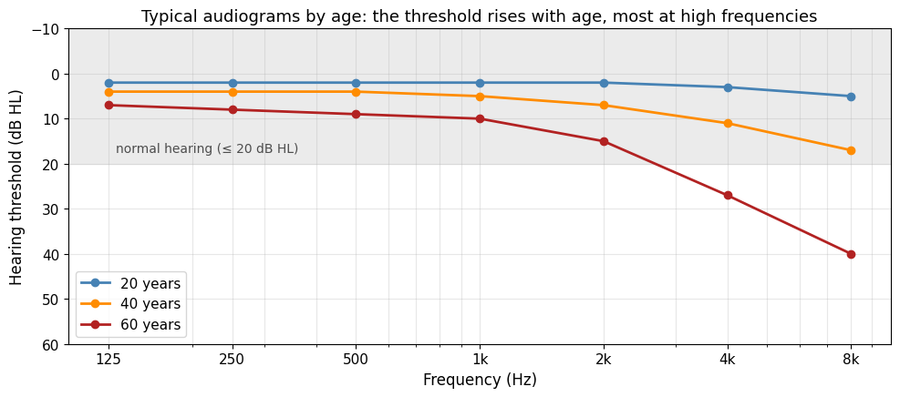
Safe listening levels
Here is a list of some different sound levels:
| Sound Source | Approximate Level (dB SPL) | Example / Context |
|---|---|---|
| Threshold of hearing | 0 | Quietest sound a healthy ear can detect |
| Rustling leaves | 10 | Very quiet, barely audible |
| Whisper | 20–30 | Soft whisper at close distance |
| Quiet library | 30–40 | Typical background noise |
| Normal conversation | 60 | At 1 metre distance |
| Busy street traffic | 70–85 | Inside a car with windows closed |
| Subway train | 95–100 | Inside the train |
| Rock concert | 110–120 | Near speakers |
| Threshold of pain | 130 | Jet engine at 30 metres |
| Fireworks / Gunshot | 140–150 | Close range |
As a rule of thumb, prolonged exposure to sounds above 85 dB can damage hearing. Typical conversation is around 60 dB, city traffic can reach 85 dB, and concerts or clubs often exceed 100 dB. The louder the sound, the shorter the safe exposure time. At 100 dB, damage can set in within about 15 minutes.
The World Health Organization (WHO) recommends keeping personal listening devices below 80 dB for adults (75 dB for children) and limiting time in loud environments. Ear protection in noisy settings and regular listening breaks both help.
Sounds above 120–130 dB, such as a jet engine at close range or fireworks, can cause immediate pain and permanent hearing loss. Even brief exposure to extremely loud sounds can irreversibly damage the hair cells in the inner ear.
Tinnitus and hearing health
Tinnitus is the perception of sound, typically a ringing, hissing, or buzzing, when no external sound is present. Many people notice a temporary version after a loud concert, often together with a muffled feeling called a temporary threshold shift, a short-lived drop in hearing sensitivity while the ear recovers. With repeated overexposure the shift can become permanent, because the hair cells of the inner ear do not grow back once destroyed (see noise-induced hearing loss). Musicians are a risk group. Surveys of rock, pop, and orchestral musicians alike find more tinnitus and hearing loss than in the general population, simply because rehearsals and concerts add up to many hours above 85 dB.
The practical response is hearing protection, of which there are many different types. Ordinary foam earplugs dampen high frequencies much more than low ones, which makes music sound dull and distant. Musicians’ earplugs instead offer flat attenuation, reducing all frequencies by roughly the same amount, typically 10–20 dB, so the mix keeps its balance and simply becomes quieter. Filtered plugs cost little, and custom-moulded versions are a sensible investment for anyone who rehearses or performs regularly.
Some ringing after a loud night is common and usually fades. If tinnitus lasts more than a day or two, or if hearing still feels muffled once the sound has stopped, book a hearing test with a doctor or audiologist. Persistent tinnitus cannot yet be cured, but it can be assessed and managed, and an early check protects the hearing you still have.
Just noticeable differences for loudness
The just noticeable difference (JND) is the smallest change in a physical stimulus that a listener can reliably detect. For loudness, it is the smallest change in sound intensity that we hear as a change in loudness.
The JND for loudness is often given as a percentage of the original level. For mid-level sounds it is typically about 1 dB, so most people need at least a 1 dB change to notice a difference. The exact value depends on the frequency, the absolute loudness, and the listening environment.
Pitch
When we hear tonal sounds—musical instruments, but also voices—we usually hear a pitch. This is closely tied to frequency, the rate at which a sound wave vibrates, but it is ultimately a subjective experience shaped by the auditory system.
Pitch range
The audible range for humans runs from roughly 20 Hz to 20,000 Hz. Sounds below 20 Hz are infrasound and generally beyond our hearing, while those above 20,000 Hz are ultrasound and also lie outside our range. Within the audible spectrum, our sensitivity to pitch varies, and is sharpest in the mid-frequency range that matters most for speech and music.
The figure below draws this range as the auditory area: everything between the threshold of hearing at the bottom and the threshold of pain at the top, on a logarithmic frequency axis from 20 Hz to 20 kHz. The two shaded regions show roughly where speech and music live within it. Speech occupies a fairly narrow band in the middle, while music spreads much wider in both frequency and level.
Source
import numpy as np
import matplotlib.pyplot as plt
plt.rcParams.update({
    "font.size": 10,
    "axes.titlesize": 11,
    "axes.labelsize": 10,
    "xtick.labelsize": 9,
    "ytick.labelsize": 9,
    "legend.fontsize": 9,
    "figure.figsize": (10, 4),
    "figure.dpi": 100,
    "savefig.dpi": 150,
    "axes.spines.top": False,
    "axes.spines.right": False,
})

# Threshold of hearing (ISO 226:2003), extended with a steep rise towards 20 kHz
f_thr = np.array([20, 25, 31.5, 40, 50, 63, 80, 100, 125, 160, 200, 250, 315, 400, 500, 630, 800,
                  1000, 1250, 1600, 2000, 2500, 3150, 4000, 5000, 6300, 8000, 10000, 12500, 14000, 16000, 18000, 20000])
t_thr = np.array([78.5, 68.7, 59.5, 51.1, 44.0, 37.5, 31.5, 26.5, 22.1, 17.9, 14.4, 11.4, 8.6, 6.2, 4.4,
                  3.0, 2.2, 2.4, 3.5, 1.7, -1.3, -4.2, -6.0, -5.4, -1.5, 6.0, 12.6, 13.9, 12.3, 22, 40, 58, 75])
# Threshold of pain: roughly 120 dB at the extremes and just under 140 dB in the middle (approximate)
f_pain = np.array([20, 50, 100, 200, 500, 1000, 2000, 5000, 10000, 15000, 20000])
t_pain = np.array([120, 129, 134, 136, 137, 137, 137, 135, 130, 122, 110])

f = np.logspace(np.log10(20), np.log10(20000), 400)
thr = np.interp(np.log10(f), np.log10(f_thr), t_thr)
pain = np.interp(np.log10(f), np.log10(f_pain), t_pain)

fig, ax = plt.subplots(figsize=(10, 5.5))
ax.set_xscale('log')
ax.fill_between(f, thr, pain, color='0.95', zorder=0)
ax.plot(f, thr, color='0.25', linewidth=2)
ax.plot(f, pain, color='0.25', linewidth=2)

def region(fc, dbc, octaves, db_span, tilt, color, label, label_at, z):
    """Tilted ellipse drawn in (log frequency, dB) space: centre fc/dbc, width in octaves, height in dB."""
    a = np.linspace(0, 2 * np.pi, 200)
    x = 0.5 * np.log10(2 ** octaves) * np.cos(a)
    y = 0.5 * db_span * np.sin(a)
    y = y + tilt * x / np.log10(2)          # tilt: dB change per octave along the long axis
    ax.fill(10 ** (np.log10(fc) + x), dbc + y, color=color, alpha=0.9, zorder=z, linewidth=0)
    ax.text(label_at[0], label_at[1], label, ha='center', va='center',
            color='white', fontweight='bold', zorder=z + 1)

region(600, 55, 7.5, 55, -4, '#7fa7c9', 'music', (150, 68), 2)    # about 45 Hz – 10 kHz, 20 – 90 dB
region(900, 52, 4.8, 32, -4, '#1f4e79', 'speech', (900, 52), 3)   # about 150 Hz – 6 kHz, 30 – 75 dB

ax.text(700, 6, 'threshold of hearing', color='0.25', ha='center', rotation=-8)
ax.text(700, 128, 'threshold of pain', color='0.25', ha='center')
ax.text(23, 100, 'infrasound\nbelow 20 Hz', color='0.4', ha='left')
ax.text(17000, 100, 'ultrasound\nabove 20 kHz', color='0.4', ha='right')
ax.set_xlim(20, 20000)
ax.set_ylim(-10, 145)
ax.set_xticks([20, 50, 100, 200, 500, 1000, 2000, 5000, 10000, 20000])
ax.set_xticklabels(['20', '50', '100', '200', '500', '1k', '2k', '5k', '10k', '20k'])
ax.set_xlabel('Frequency (Hz)')
ax.set_ylabel('Sound pressure level (dB SPL)')
ax.set_title('The auditory area: what humans can hear, and where speech and music sit within it')
ax.grid(True, which='both', alpha=0.3)
plt.tight_layout()
plt.show()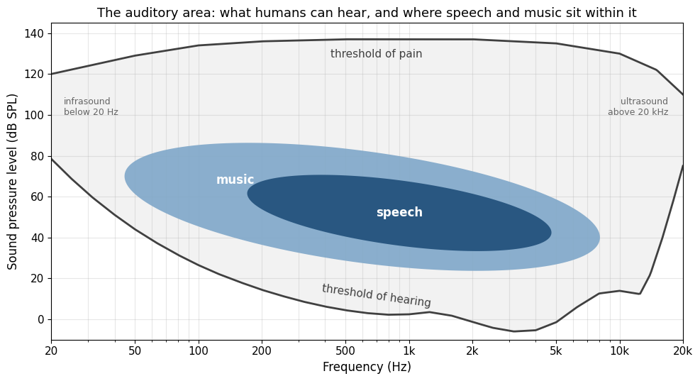
Dogs are well known for hearing better than humans, and the chart below shows that human hearing sits in the middle of the animal range. Different species have evolved to detect the frequencies most relevant to their survival and communication. Dogs can hear up to around 45,000 Hz, picking up high-pitched sounds we cannot. Bats and dolphins perceive even higher frequencies, well into the ultrasonic range, which they use for echolocation. Elephants and some whales, on the other hand, hear infrasound—very low frequencies below our threshold—which helps them communicate over long distances.
The chart below compares the approximate hearing ranges of a selection of animals, sorted by their upper limit, with the human range shaded. The differences reflect the ecological needs and evolutionary pressures each species has faced: fish and frogs live in a low-frequency world, small mammals such as mice hear far into the ultrasonic range, and the echolocators, bats and dolphins, reach highest of all.
Source
import numpy as np
import matplotlib.pyplot as plt
plt.rcParams.update({
    "font.size": 10,
    "axes.titlesize": 11,
    "axes.labelsize": 10,
    "xtick.labelsize": 9,
    "ytick.labelsize": 9,
    "legend.fontsize": 9,
    "figure.figsize": (10, 4),
    "figure.dpi": 100,
    "savefig.dpi": 150,
    "axes.spines.top": False,
    "axes.spines.right": False,
})

# Approximate hearing ranges (Hz) at moderate level, after Heffner & Heffner and Fay (1988)
species = [
    ('Goldfish',            20,     3000),
    ('Bullfrog',           100,     3000),
    ('Chicken',            125,     2000),
    ('Elephant',            16,    12000),
    ('Barn owl',           200,    12000),
    ('Human',               20,    20000),
    ('Horse',               55,    33500),
    ('Cow',                 23,    35000),
    ('Rabbit',             360,    42000),
    ('Dog',                 67,    45000),
    ('Cat',                 45,    64000),
    ('Mouse',             1000,    91000),
    ('Little brown bat', 10000,   115000),
    ('Beluga whale',      1000,   123000),
    ('Bottlenose dolphin', 150,   150000),
]
species.sort(key=lambda s: s[2])   # lowest upper limit at the bottom

def fmt(hz):
    return f'{hz / 1000:g} kHz' if hz >= 1000 else f'{hz:g} Hz'

fig, ax = plt.subplots(figsize=(10, 6.5))
ax.set_xscale('log')
ax.axvspan(20, 20000, color='0.93', zorder=0)
ax.axvline(20, color='grey', linestyle=':', linewidth=1)
ax.axvline(20000, color='grey', linestyle=':', linewidth=1)
for y, (name, lo, hi) in enumerate(species):
    color = 'darkorange' if name == 'Human' else 'steelblue'
    ax.barh(y, hi - lo, left=lo, height=0.55, color=color)
    ax.text(hi * 1.15, y, f'{fmt(lo)} – {fmt(hi)}', va='center', color='0.3')
ax.set_yticks(range(len(species)))
ax.set_yticklabels([s[0] for s in species])
ax.get_yticklabels()[[s[0] for s in species].index('Human')].set_fontweight('bold')
ax.set_xlim(8, 1.5e6)
ax.set_xticks([10, 100, 1000, 10000, 100000])
ax.set_xticklabels(['10 Hz', '100 Hz', '1 kHz', '10 kHz', '100 kHz'])
ax.text(14, len(species) - 0.4, 'infrasound', ha='right', color='0.4')
ax.text(28000, len(species) - 0.4, 'ultrasound', ha='left', color='0.4')
ax.text(630, len(species) - 0.4, 'human range', ha='center', color='0.4')
ax.set_xlabel('Frequency')
ax.set_title('Approximate hearing ranges of selected animals')
ax.grid(True, axis='x', which='both', alpha=0.3)
plt.tight_layout()
plt.show()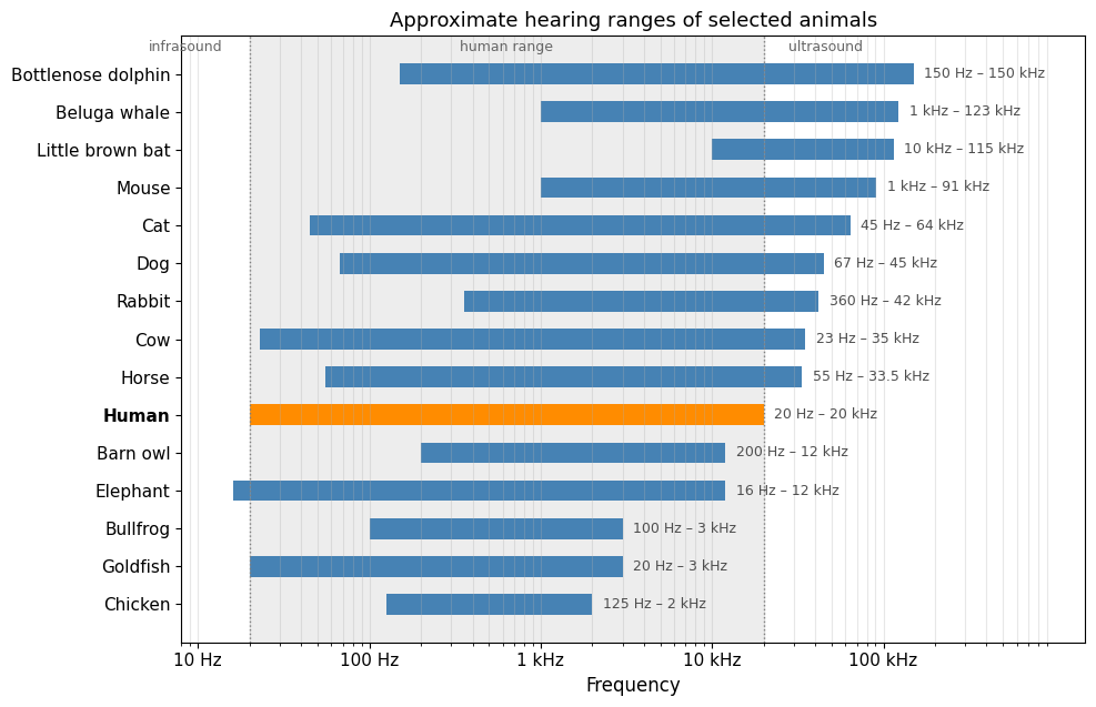
Just noticeable differences for pitch
There is a just noticeable difference (JND) for pitch too: the smallest change in frequency a listener can reliably detect. The ear is highly sensitive to small frequency changes, especially in the mid range (about 500–4000 Hz, where speech and music are most prominent). At 1000 Hz, the JND for pitch is typically around 3 Hz for trained listeners, about 0.3% of the frequency. In other words, play two tones at 1000 Hz and 1003 Hz and a trained listener can usually tell them apart. At very low or very high frequencies the JND grows larger, so small pitch differences become harder to hear.
The JND for pitch varies with factors such as the listener’s age, hearing ability, and training, the loudness of the tones, and whether the tones are heard in isolation or in a complex sound environment.
Timbre
Timbre is the quality of a sound that lets us tell different sources apart even when they share the same pitch and loudness. It is what distinguishes a piano from a violin playing the same note at the same volume. Timbre comes from the spectral content (the mix of the fundamental and the overtones), the temporal envelope (attack, decay, sustain, release), and other features such as vibrato or noise components. In music, it is how we identify instruments, voices, and textures.
Overtones
A note from an instrument or voice is a whole set of partials, the fundamental plus a series of higher overtones, and the pattern and strength of those overtones is what gives the sound its colour. The terminology, and what the overtone series looks like for different waveforms, is covered in the acoustics and electroacoustics chapters. The perceptual question is a different one: how much of that series does the ear actually need?
Envelope
The envelope of a sound is how its level unfolds over time: how it starts, develops, and ends. The electroacoustics chapter shows the standard ADSR model and how synthesisers use it to shape notes. For perception the important part is the start. The attack is the strongest single cue we have for recognising an instrument: it carries the noise of the bow striking the string, the breath before a flute tone settles, or the hammer hitting a piano string. Cut the first few tens of milliseconds off a recorded note and listeners find it surprisingly hard to say whether a piano, a trumpet, or a guitar played it, even though the sustained part of the sound is untouched. Play a piano note backwards, so that it swells instead of striking, and it no longer sounds like a piano at all. Spectral content tells us what kind of sound it is; the envelope tells us what made it.
Just noticeable differences of timbre
How many partials do you need to recognise the timbre of a sound? Below you can find examples of a Sonny Rollins saxophone tone that has been spectrally decomposed and then resynthesised with an increasing number of overtones. Each resynthesis keeps the harmonics up to a fixed point and discards the rest, so its spectrum falls off a cliff; the code finds that cliff and labels the players with the harmonic number where it sits. The series roughly doubles at each step and stops once it reaches the band limit of the recording itself, beyond which adding partials changes nothing. How many overtones do you need to hear the full richness of the saxophone?
Source
import librosa
import numpy as np
from pathlib import Path
import matplotlib.pyplot as plt
plt.rcParams.update({
    "font.size": 10,
    "axes.titlesize": 11,
    "axes.labelsize": 10,
    "xtick.labelsize": 9,
    "ytick.labelsize": 9,
    "legend.fontsize": 9,
    "figure.figsize": (10, 4),
    "figure.dpi": 100,
    "savefig.dpi": 150,
    "axes.spines.top": False,
    "axes.spines.right": False,
})

# The resyntheses of one saxophone tone, each adding more of the overtone
# series on top of the fundamental. The last file of the set is dropped: it
# duplicates the one before it, since both already reach the band limit of
# the recording.
examples = sorted(Path("audio").glob("rollins_ex16?.wav"))[:-1]

f0 = 210.0          # fundamental of the analysed tone, in Hz
n_fft = 16384

spectra, partial_counts = [], []
for path in examples:
    y, sr = librosa.load(path, sr=None, mono=True)
    mag = np.abs(librosa.stft(y, n_fft=n_fft)).mean(axis=1)
    freqs = librosa.fft_frequencies(sr=sr, n_fft=n_fft)
    db = librosa.amplitude_to_db(mag, ref=mag.max())
    spectra.append((freqs, db))
    # Level of each harmonic of the fundamental, read off the spectrum.
    levels = np.array([db[(freqs > n * f0 - 25) & (freqs < n * f0 + 25)].max()
                       for n in range(1, 105)])
    # The resynthesis stops at a fixed harmonic, so the number of partials is
    # where the series falls off a cliff: the largest one-harmonic drop.
    partial_counts.append(int(np.argmin(np.diff(levels))) + 1)

fig, axes = plt.subplots(2, 4, figsize=(11, 5.5), sharex=True, sharey=True)
for ax, (freqs, db), n, path in zip(axes.ravel(), spectra, partial_counts, examples):
    ax.plot(freqs, db, linewidth=0.8)
    ax.set_xscale('log')
    ax.set_xlim(150, 22000)
    ax.set_ylim(-80, 5)
    ax.set_title(f"{n} partial{'s' if n > 1 else ''}")
    ax.grid(alpha=0.3)
for ax in axes[-1]:
    ax.set_xlabel("Frequency (Hz)")
for ax in axes[:, 0]:
    ax.set_ylabel("Level (dB)")
fig.suptitle("One saxophone tone, resynthesised with a growing overtone series")
fig.tight_layout()
plt.show()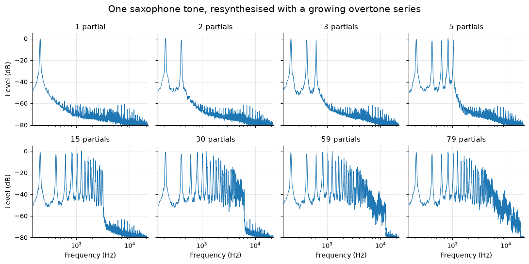
Source
from IPython.display import display, Audio

for path, n in zip(examples, partial_counts):
    print(f"{n} partial{'s' if n > 1 else ''} ({path.name}):")
    y, sr = librosa.load(path, sr=None, mono=True)
    display(Audio(y, rate=sr))
1 partial (rollins_ex16a.wav):
2 partials (rollins_ex16b.wav):
3 partials (rollins_ex16c.wav):
5 partials (rollins_ex16d.wav):
15 partials (rollins_ex16e.wav):
30 partials (rollins_ex16f.wav):
59 partials (rollins_ex16g.wav):
79 partials (rollins_ex16h.wav):
Spatial perception
Spatial hearing is our ability to perceive where sound sources are and how they move. It lets us judge whether a sound is in front, behind, above, below, or to the side. We rely on it to navigate, to follow speech in busy settings, and to enjoy immersive audio in music and virtual reality.
Binaural hearing is the use of both ears together to pick up spatial cues and locate sounds. By comparing differences in timing (ITD) and intensity (ILD) between the two ears, the brain builds a three-dimensional auditory scene. This is what gives us depth, localisation, and the ability to separate sources in a complex environment.
Interaural time difference
The interaural time difference (ITD) is the difference in the arrival time of a sound at each ear. When a source is off-centre, the sound reaches one ear slightly before the other. The brain uses this tiny gap, especially for low-frequency sounds, to locate the direction of the source on the horizontal plane. ITD is a primary cue for the azimuth (left-right position) of a sound.
The figure below shows a click from a source on the right as it arrives at the two ears. The left ear receives it about 0.6 ms later, which is close to the largest delay the human head can produce.
Source
import numpy as np
import matplotlib.pyplot as plt
plt.rcParams.update({
    "font.size": 10,
    "axes.titlesize": 11,
    "axes.labelsize": 10,
    "xtick.labelsize": 9,
    "ytick.labelsize": 9,
    "legend.fontsize": 9,
    "figure.figsize": (10, 4),
    "figure.dpi": 100,
    "savefig.dpi": 150,
    "axes.spines.top": False,
    "axes.spines.right": False,
})

# A short low-frequency click reaching the two ears from a source on the right.
# The far (left) ear receives it about 0.6 ms later: the interaural time difference.
sr = 96000
t = np.arange(0, 0.006, 1 / sr)
itd = 0.0006                                   # seconds, source roughly 60 degrees to the right
def click(delay):
    tt = t - delay
    return np.where(tt >= 0, np.sin(2 * np.pi * 500 * tt) * np.exp(-tt / 0.0012), 0)

right, left = click(0.001), click(0.001 + itd)
fig, axes = plt.subplots(2, 1, figsize=(10, 4.5), sharex=True, sharey=True)
for ax, sig, name, color in zip(axes, [right, left], ['Right ear (near)', 'Left ear (far)'], ['steelblue', 'darkorange']):
    ax.plot(t * 1000, sig, color=color, linewidth=1.8)
    ax.axhline(0, color='0.7', linewidth=0.6)
    ax.set_ylabel(name)
    ax.set_yticks([])
    ax.grid(alpha=0.3)
for ax in axes:
    ax.axvline(1.0, color='grey', linestyle=':', linewidth=1)
    ax.axvline(1.0 + itd * 1000, color='grey', linestyle=':', linewidth=1)
axes[0].annotate('', xy=(1.0 + itd * 1000, 0.85), xytext=(1.0, 0.85), arrowprops=dict(arrowstyle='<->', color='0.3'))
axes[0].text(1.0 + itd * 500, 0.95, f'ITD = {itd * 1e6:.0f} µs', ha='center', color='0.3')
axes[1].set_xlabel('Time (ms)')
axes[0].set_ylim(-1.1, 1.25)
plt.suptitle('Interaural time difference: a click from the right reaches the left ear later')
plt.tight_layout()
plt.show()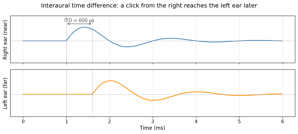
Interaural level difference
The interaural level difference (ILD) is the difference in sound pressure level reaching each ear. When a sound comes from one side, the head acts as a barrier, so the sound is louder in the near ear and quieter in the far ear. ILD works best for high-frequency sounds, where this head-shadow effect is more pronounced. The brain combines ILD with ITD to locate sounds accurately. With headphones on, you can hear the two cues separately in the Spatial hearing app, which moves a source around a schematic head with ITD and ILD switchable on and off.
The figure below shows a short noise burst from a source on the right as the two ears receive it. The left ear, turned away from the source, gets a weaker and duller version, since the head blocks the high frequencies far more than the low ones.
Source
import numpy as np
from scipy.signal import butter, lfilter
import matplotlib.pyplot as plt
plt.rcParams.update({
    "font.size": 10,
    "axes.titlesize": 11,
    "axes.labelsize": 10,
    "xtick.labelsize": 9,
    "ytick.labelsize": 9,
    "legend.fontsize": 9,
    "figure.figsize": (10, 4),
    "figure.dpi": 100,
    "savefig.dpi": 150,
    "axes.spines.top": False,
    "axes.spines.right": False,
})

# A broadband noise burst from a source on the right. The head shadows the far ear,
# so the left ear receives a weaker and duller version: the interaural level difference.
sr = 44100
rng = np.random.default_rng(1)
t = np.arange(0, 0.12, 1 / sr)
env = np.clip(t / 0.005, 0, 1) * np.exp(-np.clip(t - 0.005, 0, None) / 0.04)
burst = rng.standard_normal(len(t)) * env
right = burst / np.abs(burst).max()
b, a = butter(2, 1500 / (sr / 2), 'low')          # the head shadow removes mostly high frequencies
shadowed = lfilter(b, a, right)
left = 10 ** (-10 / 20) * shadowed / np.abs(shadowed).max()   # about 10 dB quieter at the far ear

fig, axes = plt.subplots(1, 2, figsize=(10, 3.8), sharey=True)
for ax, sig, name, color in zip(axes, [left, right], ['Left ear (far)', 'Right ear (near)'], ['darkorange', 'steelblue']):
    ax.plot(t * 1000, sig, color=color, linewidth=0.8)
    ax.set_title(name)
    ax.set_xlabel('Time (ms)')
    ax.set_ylim(-1.1, 1.1)
    ax.grid(alpha=0.3)
axes[0].set_ylabel('Amplitude')
axes[0].text(60, 0.85, 'about 10 dB weaker\nand duller', ha='center', color='0.3')
plt.suptitle('Interaural level difference: the head shadows the ear turned away from the source')
plt.tight_layout()
plt.show()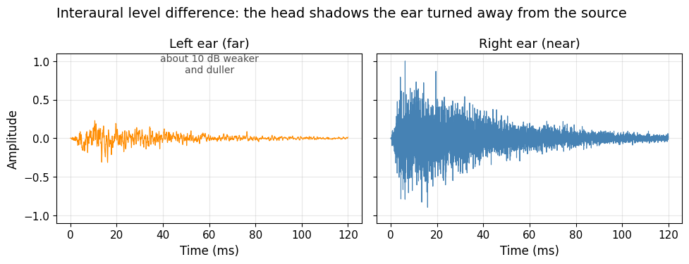
Head-related transfer function
The head-related transfer function (HRTF) describes how an ear receives a sound from a particular point in space, taking into account the effects of the listener’s head, torso, and outer ear (pinna). HRTFs are unique to each individual and are key to perceiving elevation and front-back differences. They are widely used in 3D audio and virtual reality to simulate realistic spatial sound.
The figure below sketches the idea for a source to the right. The near ear receives the sound directly, while the far ear receives it later and with the high frequencies weakened by the head, and the folds of each outer ear carve notches into the spectrum whose positions depend on where the sound comes from. The HRTF is the whole of that filtering, one pair of curves for every direction, and it is what a binaural rendering applies to a mono signal to place it in space.
Source
import numpy as np
from matplotlib.patches import Circle, Polygon, FancyArrowPatch
import matplotlib.pyplot as plt
plt.rcParams.update({
    "font.size": 10,
    "axes.titlesize": 11,
    "axes.labelsize": 10,
    "xtick.labelsize": 9,
    "ytick.labelsize": 9,
    "legend.fontsize": 9,
    "figure.figsize": (10, 4),
    "figure.dpi": 100,
    "savefig.dpi": 150,
    "axes.spines.top": False,
    "axes.spines.right": False,
})

# Schematic head-related transfer functions for a source 45 degrees to the right (not measured data)
f = np.logspace(np.log10(100), np.log10(16000), 500)
def shelf(freq, fc, gain_db):
    return gain_db / (1 + (fc / freq) ** 2)                       # smooth high-frequency shelf
def notch(freq, fc, depth_db, width=0.12):
    return -depth_db * np.exp(-((np.log10(freq) - np.log10(fc)) / width) ** 2)
right = shelf(f, 2000, 4) + notch(f, 8500, 14)                    # near ear: slight boost, pinna notch
left = shelf(f, 1500, -12) + notch(f, 7000, 8) + notch(f, 12000, 6)   # far ear: head shadow, weaker notches

fig, (ax1, ax2) = plt.subplots(1, 2, figsize=(10, 3.8), gridspec_kw={'width_ratios': [1, 1.4]})

# --- left: top-down view ---
ax1.set_aspect('equal'); ax1.axis('off'); ax1.set_xlim(-2.4, 2.4); ax1.set_ylim(-2.0, 2.4)
ax1.add_patch(Circle((0, 0), 1.0, facecolor='0.92', edgecolor='0.3', linewidth=2))
ax1.add_patch(Polygon([[-0.25, 0.97], [0, 1.3], [0.25, 0.97]], closed=False, fill=False, edgecolor='0.3', linewidth=2))
for x, color in ((-1.0, 'darkorange'), (1.0, 'steelblue')):
    ax1.add_patch(Circle((x, 0), 0.2, facecolor='white', edgecolor=color, linewidth=2.5))
src = (1.5, 1.5)
ax1.plot(*src, 'o', color='0.2', markersize=12)
ax1.text(src[0] + 0.15, src[1] + 0.2, 'source, 45° right', fontsize=10, color='0.2')
ax1.add_patch(FancyArrowPatch(src, (1.2, 0.15), arrowstyle='->', color='steelblue', linewidth=2, mutation_scale=15))
ax1.add_patch(FancyArrowPatch(src, (-1.15, 0.2), arrowstyle='->', color='darkorange', linewidth=2, linestyle='--',
                              mutation_scale=15, connectionstyle='arc3,rad=-0.55'))
ax1.text(1.3, -0.55, 'near ear:\ndirect path', fontsize=10, color='steelblue', ha='center', va='top')
ax1.text(-1.3, -0.55, 'far ear:\naround the head,\nlater and shadowed', fontsize=10, color='darkorange', ha='center', va='top')
ax1.text(0, 1.45, 'front', fontsize=9, color='0.4', ha='center')
ax1.set_title('One source, two very different signals')

# --- right: what each ear receives ---
ax2.semilogx(f, right, color='steelblue', linewidth=2, label='right ear (near)')
ax2.semilogx(f, left, color='darkorange', linewidth=2, label='left ear (far)')
ax2.axhline(0, color='0.7', linewidth=0.8)
ax2.fill_between(f, left, right, where=f > 1500, color='0.93', zorder=0)
ax2.annotate('head shadow:\nlevel difference (ILD)', xy=(4000, -5), xytext=(1400, -20),
             arrowprops=dict(arrowstyle='->', color='0.4'), fontsize=10, color='0.3')
ax2.annotate('pinna notch: its frequency\nshifts with elevation and\nfront versus back', xy=(8500, -10), xytext=(2600, -32),
             arrowprops=dict(arrowstyle='->', color='0.4'), fontsize=10, color='0.3')
ax2.text(110, 4, 'low frequencies bend around the head:\nboth ears hear the same level', fontsize=10, color='0.3', va='bottom')
ax2.set_xlim(100, 16000)
ax2.set_ylim(-36, 12)
ax2.set_xticks([100, 200, 500, 1000, 2000, 5000, 10000])
ax2.set_xticklabels(['100', '200', '500', '1k', '2k', '5k', '10k'])
ax2.set_xlabel('Frequency (Hz)')
ax2.set_ylabel('Level relative to free field (dB)')
ax2.set_title('Head-related transfer function for that direction (schematic)')
ax2.legend(loc='lower left')
ax2.grid(True, which='both', alpha=0.3)
plt.tight_layout()
plt.show()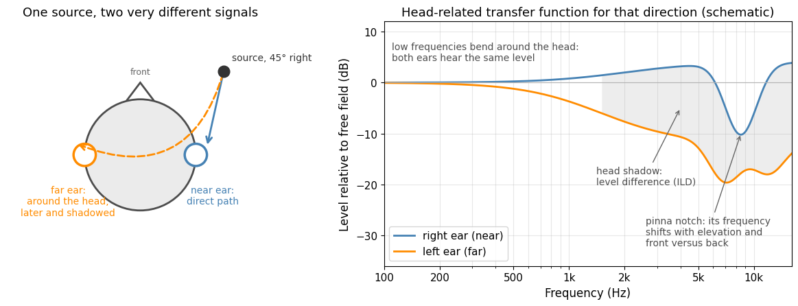
The precedence effect is a phenomenon where the first-arriving sound dominates our sense of where the sound is, even when reflections or echoes follow shortly after. It helps us lock onto the direct source in reverberant spaces, such as a speaker’s voice in a large hall, rather than getting confused by reflections.
Cocktail party effect
The cocktail party effect is our ability to focus on a single sound source, such as a conversation partner, in a noisy environment full of competing sounds. This selective attention draws on spatial hearing cues as well as cognitive processes to filter out background noise and bring out the target sound. It is a central part of auditory scene analysis and of how we manage to communicate in social settings.
Auditory scene analysis
Everything so far has concerned single sounds: one tone’s loudness, one tone’s pitch, one source’s location. Real listening is almost never like that. At any moment the eardrum receives one pressure wave that is the sum of every sound source in the room. Somehow we hear a singer, a guitar, a passing car and a fan, not one blended smear.
The Canadian psychologist Albert Bregman (1936–2023) named this problem auditory scene analysis (ASA) in his 1990 book of the same title Bregman, 1990. The auditory system has to solve two grouping problems at once:
- Simultaneous grouping decides which frequency components belong to the same sound right now. Partials that start together, share a harmonic relationship, and change together tend to fuse into one tone, which is why we hear a single trumpet note rather than a dozen separate partials.
- Sequential grouping decides which sounds belong to the same source over time. Sounds that are close in pitch, timbre, and location, and follow each other at a moderate rate, tend to bind into a single stream.
Bregman’s cues are the hearing versions of the Gestalt principles that psychologists first described for vision a century ago: things that are close together (proximity), that resemble each other (similarity), that change together (common fate), and that continue smoothly (good continuation) are seen, and heard, as belonging together. Sounds close in pitch and time group by proximity, sounds of one timbre by similarity, partials that rise and fall together by common fate. The principles themselves, with a figure, are taken up in harmony and melody, where they explain how we hear voices in a texture. Here we look at the three basic effects, one at a time, each with a figure and a sound.
Simultaneous grouping
The strongest cue that partials belong to one sound is that they start at the same moment. In the first example below, six harmonics of 220 Hz begin together and you hear a single tone with a clear pitch; the partials have fused. In the second, one harmonic starts 0.4 s before the others. It is heard on its own before the rest arrive, and it tends to stay heard as a separate tone even once they have, because the auditory system has already assigned it to a different source. The same thing happens when one partial is slightly mistuned from the harmonic series or is modulated differently from the rest.
Source
import numpy as np
from IPython.display import Audio, display
import matplotlib.pyplot as plt
plt.rcParams.update({
    "font.size": 10,
    "axes.titlesize": 11,
    "axes.labelsize": 10,
    "xtick.labelsize": 9,
    "ytick.labelsize": 9,
    "legend.fontsize": 9,
    "figure.figsize": (10, 4),
    "figure.dpi": 100,
    "savefig.dpi": 150,
    "axes.spines.top": False,
    "axes.spines.right": False,
})

# Simultaneous grouping: six harmonics of 220 Hz, either starting together or with one starting early
sr = 22050
f0, harmonics, dur, lead = 220, [1, 2, 3, 4, 5, 6], 1.5, 0.4
early = 4                                              # the harmonic that starts early in the second example

def tone(start_times):
    n = int(sr * dur); t = np.arange(n) / sr; y = np.zeros(n)
    for h, t0 in zip(harmonics, start_times):
        env = np.clip((t - t0) / 0.01, 0, 1) * np.clip((dur - t) / 0.01, 0, 1)
        y += env * np.sin(2 * np.pi * h * f0 * t) / h
    return 0.4 * y / np.abs(y).max()

together = [0.0] * len(harmonics)
staggered = [0.0 if h == early else lead for h in harmonics]

fig, axes = plt.subplots(1, 2, figsize=(10, 3.2), sharey=True)
for ax, starts, title in zip(axes, [together, staggered], ['All partials start together: heard as one tone',
                                                            'One partial starts early: it is heard on its own']):
    for h, t0 in zip(harmonics, starts):
        color = 'darkorange' if (h == early and starts is staggered) else 'steelblue'
        ax.hlines(h * f0, t0, dur, color=color, linewidth=4)
    ax.set_xlim(-0.05, dur); ax.set_ylim(0, 7.2 * f0)
    ax.set_yticks([h * f0 for h in harmonics]); ax.set_yticklabels([f'{h * f0}' for h in harmonics])
    ax.set_xlabel('Time (s)'); ax.set_title(title); ax.grid(alpha=0.3)
axes[0].set_ylabel('Frequency (Hz)')
axes[1].annotate('starts 0.4 s early', xy=(0.02, early * f0), xytext=(0.25, 6.6 * f0),
                 arrowprops=dict(arrowstyle='->', color='0.4'), color='0.3')
plt.suptitle('Simultaneous grouping: partials that start together fuse into one sound')
plt.tight_layout(); plt.show()

print("Six harmonics starting together: one tone.")
display(Audio(tone(together), rate=sr))
print(f"The same six harmonics, but the {early}th (880 Hz) starts 0.4 s early: listen for it as a separate tone that stays separate.")
display(Audio(tone(staggered), rate=sr))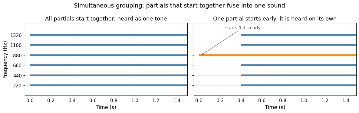
Six harmonics starting together: one tone.
The same six harmonics, but the 4th (880 Hz) starts 0.4 s early: listen for it as a separate tone that stays separate.
Sequential grouping and streaming
The classic demonstration alternates two tones in a gallop: A–B–A–silence–A–B–A. When A and B are close in frequency, you hear one bouncing melody. Pull them apart, and the sequence splits into two streams—a fast one and a slow one—and the galloping rhythm disappears, even though not a single note has moved in time. This is stream segregation, and it shows that rhythm is a property of a stream, not of the signal. The figure below shows the two cases and the sounds follow; the dotted line marks what you hear as one line.
Streaming builds up over a few seconds and depends on rate. The faster the alternation and the wider the frequency separation, the more likely the split. Composers have exploited it for centuries. In compound melody—a solo Bach partita, say—a single instrument plays one line of notes that listeners hear as two interleaved voices.
Source
import numpy as np
from matplotlib.ticker import NullFormatter
from IPython.display import Audio, display
import matplotlib.pyplot as plt
plt.rcParams.update({
    "font.size": 10,
    "axes.titlesize": 11,
    "axes.labelsize": 10,
    "xtick.labelsize": 9,
    "ytick.labelsize": 9,
    "legend.fontsize": 9,
    "figure.figsize": (10, 4),
    "figure.dpi": 100,
    "savefig.dpi": 150,
    "axes.spines.top": False,
    "axes.spines.right": False,
})

# Sequential grouping: the A-B-A gallop with a small and a large frequency separation
sr = 22050
tone_ms, f_a = 100, 400

def gallop(f_a, f_b, n_cycles=8):
    t = np.linspace(0, tone_ms / 1000, int(sr * tone_ms / 1000), endpoint=False)
    env = np.minimum(1, np.minimum(t, t[-1] - t) / 0.01)          # 10 ms ramps
    a, b = np.sin(2 * np.pi * f_a * t) * env, np.sin(2 * np.pi * f_b * t) * env
    return np.tile(np.concatenate([a, b, a, np.zeros_like(a)]), n_cycles) * 0.3

fig, axes = plt.subplots(1, 2, figsize=(10, 3.2))
for ax, f_b, title in zip(axes, [480, 1600], ['Small separation: one galloping stream', 'Large separation: two separate streams']):
    seq = [(f_a, 0), (f_b, 1), (f_a, 2)]
    xs, ys = [], []
    for cycle in range(3):
        for f, slot in seq:
            t0 = (cycle * 4 + slot) * tone_ms / 1000
            ax.hlines(f, t0, t0 + tone_ms / 1000, color='steelblue' if f == f_a else 'darkorange', linewidth=5)
            xs.append(t0 + tone_ms / 2000); ys.append(f)
    if f_b == 480:
        ax.plot(xs, ys, color='0.5', linestyle=':', linewidth=1.5)          # one zigzag stream
    else:
        for f in (f_a, f_b):
            ax.axhline(f, color='0.5', linestyle=':', linewidth=1.5)         # two flat streams
    ax.set_yscale('log'); ax.set_ylim(300, 2200); ax.set_yticks([400, 480, 800, 1600]); ax.set_yticklabels(['400', '480', '800', '1600']); ax.yaxis.set_minor_formatter(NullFormatter())
    ax.set_xlim(-0.05, 1.2); ax.set_xlabel('Time (s)'); ax.set_title(title); ax.grid(alpha=0.3, which='both')
axes[0].set_ylabel('Frequency (Hz)')
axes[0].text(0.0, 318, 'dotted line: what you hear as one line', color='0.3')
plt.suptitle('Sequential grouping: the same rhythm, heard as one stream or two')
plt.tight_layout(); plt.show()

print("Small separation (400 / 480 Hz): one galloping stream.")
display(Audio(gallop(f_a, 480), rate=sr))
print("Large separation (400 / 1600 Hz): a fast low stream and a slow high one, and the gallop is gone.")
display(Audio(gallop(f_a, 1600), rate=sr))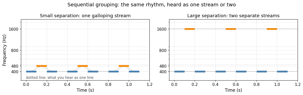
Small separation (400 / 480 Hz): one galloping stream.
Large separation (400 / 1600 Hz): a fast low stream and a slow high one, and the gallop is gone.
The continuity illusion
If a tone is interrupted by a short silence, you hear a gap. Fill that gap with a loud burst of noise instead, and the tone seems to continue right through it: the continuity illusion. The auditory system treats the noise as a plausible masker and reconstructs what was probably there. The figure below shows the two signals, and in the sounds the tone is first interrupted by silence and then by noise.
This is not a curiosity but the everyday case. Conversations survive passing traffic, and melodies survive coughs in the concert hall, because the auditory system fills in the parts that could have been masked. It is the same logic as the missing fundamental below. Perception is constructive, not a passive copy of the waveform.
Source
import numpy as np
from IPython.display import Audio, display
import matplotlib.pyplot as plt
plt.rcParams.update({
    "font.size": 10,
    "axes.titlesize": 11,
    "axes.labelsize": 10,
    "xtick.labelsize": 9,
    "ytick.labelsize": 9,
    "legend.fontsize": 9,
    "figure.figsize": (10, 4),
    "figure.dpi": 100,
    "savefig.dpi": 150,
    "axes.spines.top": False,
    "axes.spines.right": False,
})

# Continuity illusion: a tone interrupted by silence, then by a burst of noise
sr = 22050
dur, gap_ms, f_tone = 2.0, 250, 500
t = np.linspace(0, dur, int(sr * dur), endpoint=False)
tone = 0.25 * np.sin(2 * np.pi * f_tone * t)
start = int(sr * (dur - gap_ms / 1000) / 2); stop = start + int(sr * gap_ms / 1000)
mask = np.ones_like(tone); mask[start:stop] = 0
rng = np.random.default_rng(0)
noise = np.zeros_like(tone); noise[start:stop] = 0.6 * rng.normal(0, 1, stop - start)
with_gap, with_noise = tone * mask, tone * mask + noise

fig, axes = plt.subplots(2, 1, figsize=(10, 5.2), sharex=True)
for ax, sig, title, heard in zip(axes, [with_gap, with_noise],
                                 ['Tone interrupted by silence', 'Same gap filled with noise'],
                                 ['heard: tone, gap, tone', 'heard: the tone continues through the noise']):
    ax.plot(t, sig, color='steelblue', linewidth=0.5)
    ax.axvspan(start / sr, stop / sr, color='0.92', zorder=0)
    ax.set_ylim(-1.1, 1.1); ax.set_yticks([]); ax.set_ylabel('Amplitude')
    ax.set_title(title, loc='left')
    ax.text(dur - 0.03, 0.85, heard, ha='right', color='0.3')
axes[1].set_xlabel('Time (s)')
plt.suptitle('The continuity illusion: the auditory system fills in what a masker could have hidden')
plt.tight_layout(); plt.show()

print("Tone interrupted by silence: you hear a gap.")
display(Audio(with_gap, rate=sr))
print("The same gap filled with noise: the tone seems to continue through it.")
display(Audio(with_noise, rate=sr))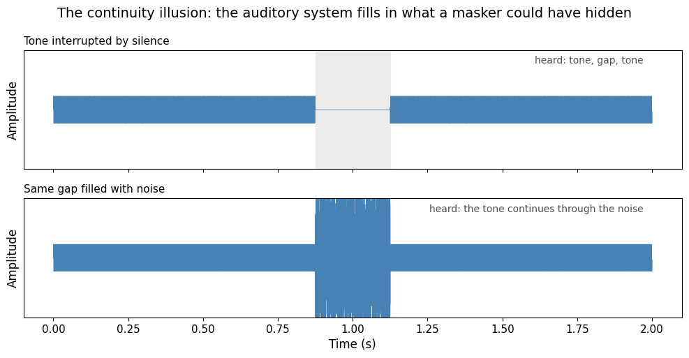
Tone interrupted by silence: you hear a gap.
The same gap filled with noise: the tone seems to continue through it.
The musical consequences of grouping, from polyphonic listening to Diana Deutsch’s illusions, are picked up in harmony and melody. The engineering counterpart, getting a machine to separate sources, appears in machine listening.
Hearing actions and objects
Auditory scene analysis explains how the incoming pressure wave is sorted into streams. But what do we hear those streams as? Rarely as frequencies and amplitudes. We hear a door slamming, a glass breaking, footsteps in the corridor: actions on objects. Researchers in sound-source perception have shown just how good listeners are at this. From sound alone, people can reliably judge the material of a struck object, its size and shape, whether a dropped bottle bounced or broke, and even the amount of liquid in a container being filled Gaver, 1993. From an ecological perspective this is unsurprising: identifying what is happening around us is what hearing is for Clarke, 2005.
This perceptual skill mirrors the action–sound couplings introduced in the acoustics chapter. Because the physics is lawful, a lifetime of interacting with objects lets us run the relationship in both directions. Watching a glass fall, we predict the crash before it lands (and may cover our ears in anticipation). Hearing a crash from the kitchen, we know a glass has broken without looking. Jensenius (2022) describes the mental image of a heard sound in three layers: an image of the action (the excitation: was the object hit, stroked, or blown into?), an image of the object (the resonance: wood, metal, or glass, large or small), and an image of the environment (the reverberation: a bathroom or a concert hall). Imagine a single drum stroke and you will find that you “hear” all three.
This is also why electro-acoustic sounds can feel detached or ambiguous. When a sound comes from a loudspeaker, there may be no mechanical action behind it at all, and the relation between control and sound is a designed action–sound mapping rather than a physical coupling (electroacoustics). Perception and cognition of sound are, in other words, not only about analysing the signal reaching the ear but about connecting it to the actions and objects that could have caused it.
Auditory illusions
The continuity illusion above is one case of a wider phenomenon. Auditory illusions show how the brain interprets sound, often departing from the raw physical signal. Studying them tells us how we organise, prioritise, and sometimes misinterpret acoustic information. That knowledge feeds into music production, audio engineering, hearing aid design, and the design of efficient audio codecs.
Hysteresis
Hysteresis is when a system’s response depends not only on its current state but also on its past states. In psychoacoustics, it turns up in loudness perception. How loud a sound seems can depend on the sounds that came before it. After a loud sound, a softer one may seem even quieter than it would in isolation. A gradual rise in volume can be perceived differently from a sudden jump, even when the final sound pressure level is the same.
The figure below sketches the idea. Turn a tone up slowly from silence and listeners report hearing it at one level; turn it down slowly from clearly audible and they keep reporting it until a lower level. The response follows two different curves depending on where it came from.
Source
import numpy as np
import matplotlib.pyplot as plt
plt.rcParams.update({
    "font.size": 10,
    "axes.titlesize": 11,
    "axes.labelsize": 10,
    "xtick.labelsize": 9,
    "ytick.labelsize": 9,
    "legend.fontsize": 9,
    "figure.figsize": (10, 4),
    "figure.dpi": 100,
    "savefig.dpi": 150,
    "axes.spines.top": False,
    "axes.spines.right": False,
})

# Schematic perceptual hysteresis: the level at which a sound is reported as heard
# is higher when the level rises from silence than when it falls from clearly audible.
spl = np.linspace(0, 40, 300)
def sigmoid(x, centre, width=4.0):
    return 100 / (1 + np.exp(-(x - centre) / width))
rising, falling = sigmoid(spl, 22), sigmoid(spl, 16)

fig, ax = plt.subplots(figsize=(10, 4.5))
ax.plot(spl, rising, color='steelblue', linewidth=2, label='level rising from silence')
ax.plot(spl, falling, color='darkorange', linewidth=2, label='level falling from clearly audible')
ax.annotate('', xy=(26, sigmoid(26, 22)), xytext=(18, sigmoid(18, 22)), arrowprops=dict(arrowstyle='->', color='steelblue', lw=2))
ax.annotate('', xy=(12, sigmoid(12, 16)), xytext=(20, sigmoid(20, 16)), arrowprops=dict(arrowstyle='->', color='darkorange', lw=2))
ax.annotate('', xy=(22, 50), xytext=(16, 50), arrowprops=dict(arrowstyle='<->', color='0.3'))
ax.text(19, 54, 'hysteresis', ha='center', color='0.3')
ax.set_xlabel('Sound pressure level (dB SPL)')
ax.set_ylabel('Reported as heard (%)')
ax.set_title('Perceptual hysteresis: where a sound is heard depends on the direction of change (schematic)')
ax.legend(loc='lower right')
ax.grid(alpha=0.3)
plt.tight_layout()
plt.show()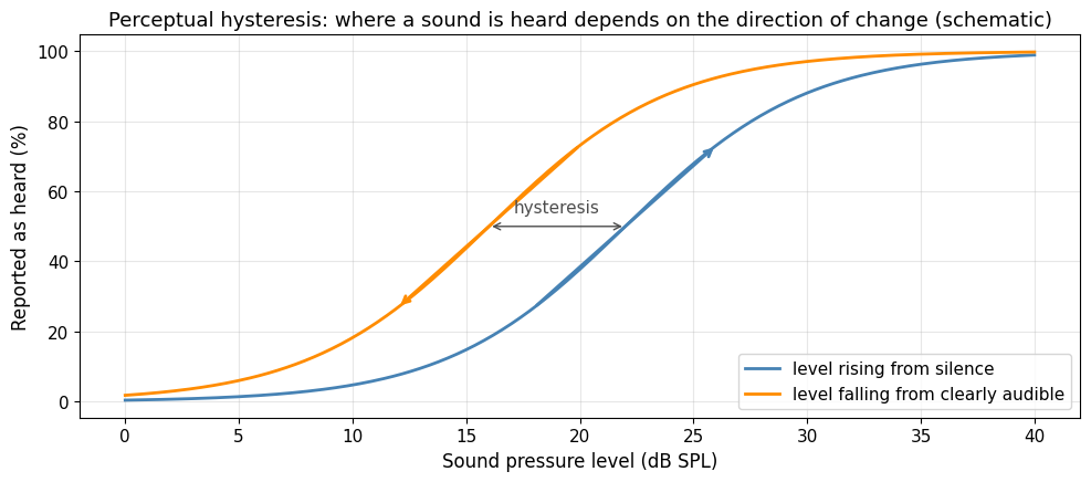
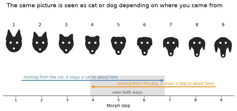
The same thing happens in vision, where it is easy to try on yourself. In the figure below, a cat silhouette is morphed into a dog in nine equal steps. Go through the row from left to right, one picture at a time, and note where the animal stops being a cat. Then start at the right-hand end and work back, noting where it stops being a dog. Most people switch late in both directions, so the pictures in the middle, which are physically identical on the two passes, get reported differently depending on which way you arrived at them.
Source
import numpy as np
import matplotlib.pyplot as plt
from scipy.interpolate import CubicSpline
plt.rcParams.update({
    "font.size": 10,
    "axes.titlesize": 11,
    "axes.labelsize": 10,
    "xtick.labelsize": 9,
    "ytick.labelsize": 9,
    "legend.fontsize": 9,
    "figure.figsize": (10, 4),
    "figure.dpi": 100,
    "savefig.dpi": 150,
    "axes.spines.top": False,
    "axes.spines.right": False,
})

# Two silhouettes described by the same landmarks in the same order, so that
# interpolating between them morphs one figure into the other.
CAT = dict(
    head=[(0.00, 0.85), (0.55, 0.72), (0.82, 0.25), (0.72, -0.30),
          (0.38, -0.68), (0.00, -0.78), (-0.38, -0.68), (-0.72, -0.30),
          (-0.82, 0.25), (-0.55, 0.72)],
    ear=[(0.18, 0.72), (0.34, 1.26), (0.56, 1.60), (0.68, 1.16), (0.78, 0.48)],
    muzzle=[(0.00, -0.14), (0.30, -0.26), (0.36, -0.52), (0.20, -0.72),
            (0.00, -0.78), (-0.20, -0.72), (-0.36, -0.52), (-0.30, -0.26)],
    eye=(0.34, 0.22, 0.10), nose=(0.0, -0.40, 0.09),
)
DOG = dict(
    head=[(0.00, 0.78), (0.44, 0.64), (0.58, 0.20), (0.50, -0.20),
          (0.30, -0.48), (0.00, -0.56), (-0.30, -0.48), (-0.50, -0.20),
          (-0.58, 0.20), (-0.44, 0.64)],
    ear=[(0.30, 0.66), (0.72, 0.42), (0.88, -0.30), (0.74, -0.80), (0.52, -0.22)],
    muzzle=[(0.00, -0.10), (0.24, -0.30), (0.25, -0.95), (0.17, -1.28),
            (0.00, -1.36), (-0.17, -1.28), (-0.25, -0.95), (-0.24, -0.30)],
    eye=(0.28, 0.20, 0.09), nose=(0.0, -1.14, 0.08),
)


def closed_spline(pts, n=400):
    """A smooth closed outline through a ring of landmarks."""
    pts = np.vstack([pts, pts[:1]])
    d = np.r_[0, np.cumsum(np.hypot(*np.diff(pts, axis=0).T))]
    return CubicSpline(d, pts, bc_type="periodic")(np.linspace(0, d[-1], n))


def draw_morph(ax, a, fg="0.15"):
    """Draw the silhouette a fraction `a` of the way from cat to dog."""
    for part, z in (("ear", 1), ("head", 2), ("muzzle", 3)):
        p = (1 - a) * np.array(CAT[part]) + a * np.array(DOG[part])
        for side in ((1, -1) if part == "ear" else (1,)):
            c = closed_spline(p * [side, 1])
            ax.fill(c[:, 0], c[:, 1], color=fg, zorder=z)
    ex, ey, er = (1 - a) * np.array(CAT["eye"]) + a * np.array(DOG["eye"])
    _, ny, nr = (1 - a) * np.array(CAT["nose"]) + a * np.array(DOG["nose"])
    for side in (1, -1):
        ax.add_patch(plt.Circle((side * ex, ey), er, color="white", zorder=4))
    ax.add_patch(plt.Circle((0, ny), nr, color="white", zorder=4))


n = 9
fig = plt.figure(figsize=(10, 3.6))
gs = fig.add_gridspec(2, n, height_ratios=[3, 1], hspace=0.05)

for i in range(n):
    ax = fig.add_subplot(gs[0, i])
    draw_morph(ax, i / (n - 1))
    ax.set_xlim(-1.15, 1.15)
    ax.set_ylim(-1.45, 1.70)
    ax.set_aspect("equal")
    ax.axis("off")
    ax.set_title(str(i + 1))

# Where the percept typically flips, scanning each way. The two points differ,
# so the pictures between them are seen as cat or dog depending on the route.
ax = fig.add_subplot(gs[1, :])
ax.axvspan(3.9, 6.8, color="0.88", zorder=0)
ax.annotate("", xy=(6.8, 0.76), xytext=(1.2, 0.76),
            arrowprops=dict(arrowstyle="-|>", color="steelblue", linewidth=2))
ax.annotate("", xy=(3.9, 0.44), xytext=(8.8, 0.44),
            arrowprops=dict(arrowstyle="-|>", color="darkorange", linewidth=2))
ax.text(1.3, 0.86, "starting from the cat, it stays a cat to about here",
        color="steelblue", fontsize=9)
ax.text(8.7, 0.54, "starting from the dog, it stays a dog to about here",
        color="darkorange", fontsize=9, ha="right")
ax.text(5.35, 0.10, "seen both ways", ha="center", fontsize=9, color="0.3")
ax.set_xlim(0.5, n + 0.5)
ax.set_ylim(0, 1)
ax.set_xticks(np.arange(1, n + 1))
ax.set_yticks([])
ax.set_xlabel("Morph step")
for side in ("left", "right", "top"):
    ax.spines[side].set_visible(False)
fig.suptitle("The same picture is seen as cat or dog depending on where you came from")
plt.show()
Grouping behaves the same way. In auditory streaming, a sequence of alternating high and low tones can be heard either as one zigzagging melody or as two separate streams, and the boundary between the two depends on which percept you started with Bregman, 1990. Widen the interval slowly and the single stream holds together past the point where it would have split; narrow it again and the two streams stay apart past the point where they would have fused. The current stimulus does not fully determine the percept: the recent past is part of the input.
Masking effects
Masking is when one sound (the masker) makes another sound (the maskee) harder to hear. The auditory system has limited frequency and temporal resolution, so a strong or similar sound can “cover up” a weaker or nearby one, making it less perceptible or even inaudible.
There are several types. In simultaneous masking, two sounds play at the same time and a louder one can render a softer one inaudible, even when both are within the listener’s hearing range. The effect is strongest when the two are close in frequency. In music production, for example, a loud bass drum can mask a softer bass guitar note if they occur together and share similar frequencies. The same principle drives audio compression formats such as MP3, which discard masked sounds to shrink file size without a noticeable loss in quality.
Frequency masking is strongest when masker and maskee are close in frequency, typically within the same critical band. The ear divides the spectrum into critical bands Fastl & Zwicker, 2007, and sounds in the same band are more likely to mask each other, which is why a high-pitched sound is unlikely to be masked by a low-pitched one, and vice versa. Masking is generally stronger for frequencies above the masker (upward spread) than below it, so a loud low-frequency sound masks higher frequencies more effectively than the reverse.
Temporal masking is when a loud sound masks a softer one that comes immediately before (pre-masking) or after (post-masking) it, even though the two do not overlap in time. Pre-masking can last up to about 20 ms before the masker, and post-masking up to about 100 ms after it. This reflects the temporal resolution limits of human hearing and is also exploited in perceptual audio coding.
The graph below shows how a masker tone, here 1 kHz at 60 dB SPL, raises the threshold of hearing for nearby frequencies, making them inaudible unless they rise above the masking threshold. A 30 dB tone at 1.3 kHz disappears under the masker, while a tone at the same level at 400 Hz is still heard, and the raised threshold reaches much further above the masker than below it. This is a key idea in psychoacoustics and audio engineering.
Source
import numpy as np
import matplotlib.pyplot as plt
plt.rcParams.update({
    "font.size": 10,
    "axes.titlesize": 11,
    "axes.labelsize": 10,
    "xtick.labelsize": 9,
    "ytick.labelsize": 9,
    "legend.fontsize": 9,
    "figure.figsize": (10, 4),
    "figure.dpi": 100,
    "savefig.dpi": 150,
    "axes.spines.top": False,
    "axes.spines.right": False,
})

# Threshold in quiet (ISO 226:2003) and the masking threshold produced by one tone
f_iso = np.array([20, 25, 31.5, 40, 50, 63, 80, 100, 125, 160, 200, 250, 315, 400, 500, 630, 800,
                  1000, 1250, 1600, 2000, 2500, 3150, 4000, 5000, 6300, 8000, 10000, 12500])
t_iso = np.array([78.5, 68.7, 59.5, 51.1, 44.0, 37.5, 31.5, 26.5, 22.1, 17.9, 14.4, 11.4, 8.6, 6.2, 4.4,
                  3.0, 2.2, 2.4, 3.5, 1.7, -1.3, -4.2, -6.0, -5.4, -1.5, 6.0, 12.6, 13.9, 12.3])
f = np.logspace(np.log10(20), np.log10(12500), 600)
quiet = np.interp(np.log10(f), np.log10(f_iso), t_iso)

def bark(freq):                                  # frequency to critical-band rate (Zwicker)
    return 13 * np.arctan(0.00076 * freq) + 3.5 * np.arctan((freq / 7500) ** 2)

masker_f, masker_L = 1000, 60                    # a 1 kHz tone at 60 dB SPL
dz = bark(f) - bark(masker_f)
spread = 15.81 + 7.5 * (dz + 0.474) - 17.5 * np.sqrt(1 + (dz + 0.474) ** 2)   # Schroeder spreading function
masking = masker_L + spread - 12                 # tone-masking-tone offset, simplified
threshold = np.maximum(quiet, masking)

fig, ax = plt.subplots(figsize=(10, 5))
ax.set_xscale('log')
ax.fill_between(f, -10, threshold, color='0.93', zorder=0)
ax.plot(f, quiet, color='0.4', linestyle='--', linewidth=1.5, label='threshold in quiet')
ax.plot(f, threshold, color='steelblue', linewidth=2, label='threshold with masker present')
ax.vlines(masker_f, -10, masker_L, color='firebrick', linewidth=6, label='masker (1 kHz, 60 dB)')
ax.vlines(1300, -10, 30, color='darkorange', linewidth=6, label='masked tone (1.3 kHz, 30 dB): inaudible')
ax.vlines(400, -10, 30, color='seagreen', linewidth=6, label='same level at 400 Hz: audible')
ax.text(2400, 14, 'upward spread\nof masking', color='0.3')
ax.text(45, 10, 'inaudible region', color='0.4')
ax.set_xlim(20, 12500)
ax.set_ylim(-10, 100)
ax.set_xticks([20, 50, 100, 200, 500, 1000, 2000, 5000, 10000])
ax.set_xticklabels(['20', '50', '100', '200', '500', '1k', '2k', '5k', '10k'])
ax.set_xlabel('Frequency (Hz)')
ax.set_ylabel('Sound pressure level (dB SPL)')
ax.set_title('Simultaneous masking: a loud tone raises the threshold for its neighbours')
ax.legend(loc='upper right')
ax.grid(True, which='both', alpha=0.3)
plt.tight_layout()
plt.show()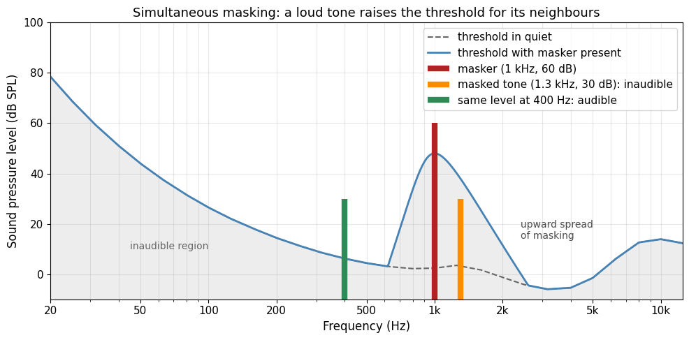
A soft tone can become inaudible when a louder sound sits close to it in frequency. Below, a quiet 1 kHz tone is played alone, then together with a band of noise centred on 1 kHz. The tone is still physically present in the second clip, but it is hard to hear. This masking is exactly what perceptual audio codecs like MP3 exploit.
Source
import numpy as np
from numpy.fft import rfft, irfft, rfftfreq
from IPython.display import Audio, display

sr = 22050
dur = 2.0
t = np.linspace(0, dur, int(sr * dur), endpoint=False)

tone = 0.05 * np.sin(2 * np.pi * 1000 * t)          # soft 1 kHz probe tone

rng = np.random.default_rng(0)                       # noise band around 1 kHz
spec = rfft(rng.standard_normal(len(t)))
freqs = rfftfreq(len(t), 1 / sr)
spec[(freqs < 700) | (freqs > 1300)] = 0
band = irfft(spec, n=len(t))
band = 0.5 * band / np.max(np.abs(band))

print("1) Soft 1 kHz tone alone:")
display(Audio(tone, rate=sr))
print("2) The same tone plus louder noise around 1 kHz (the tone is masked):")
display(Audio(tone + band, rate=sr))
print("3) The masking noise on its own:")
display(Audio(band, rate=sr))
1) Soft 1 kHz tone alone:
2) The same tone plus louder noise around 1 kHz (the tone is masked):
3) The masking noise on its own:
Masking turns up everywhere. A passing truck can mask a conversation until it has gone by. In music, masking can be used on purpose to blend instruments or to hide imperfections in a recording. In hearing aids, understanding it helps in designing algorithms that bring out speech while suppressing background noise. Masking is also the engine of lossy audio compression: a perceptual codec such as MP3 or AAC discards exactly those components its model predicts are masked, which is how streaming audio can keep a fraction of the original data without most listeners noticing (see electroacoustics).
Shepard and Risset tones
One of the best-known auditory illusions is the Shepard tone, named after Roger Shepard (1929–2022), who first described it Shepard, 1964. It is a series of tones that seem to climb or fall endlessly without ever actually getting higher or lower, the auditory equivalent of a barber pole.
A Shepard tone is built by layering several sine waves spaced an octave apart. As the sequence runs, all the sine waves move up (or down) together. The highest one fades out as it reaches the top of the range while a new, low one fades in at the bottom. The overall amplitude envelope is shaped so the listener always hears a similar blend of frequencies, with no clear start or end. This constant overlap and cross-fading make the brain hear a never-ending rise (or fall), even though the actual frequencies cycle within a fixed range. The illusion plays on the way our hearing groups harmonically related tones, which makes it hard to pin down when the scale “resets”.
The figure below shows a spectrogram of such a tone: seven components, each rising one octave every four seconds under a fixed bell-shaped envelope, so that a new one fades in at the bottom as the top one fades out. Listen to it for a while and notice that it never arrives anywhere.
Source
import numpy as np
import librosa
import librosa.display
from IPython.display import Audio, display
import matplotlib.pyplot as plt
plt.rcParams.update({
    "font.size": 10,
    "axes.titlesize": 11,
    "axes.labelsize": 10,
    "xtick.labelsize": 9,
    "ytick.labelsize": 9,
    "legend.fontsize": 9,
    "figure.figsize": (10, 4),
    "figure.dpi": 100,
    "savefig.dpi": 150,
    "axes.spines.top": False,
    "axes.spines.right": False,
})

# An endlessly rising Shepard tone: octave-spaced components under a fixed bell-shaped envelope
sr = 22050
dur = 8.0
t = np.linspace(0, dur, int(sr * dur), endpoint=False)
f0 = 55.0          # lowest reference frequency
n = 7              # number of octave-spaced components
period = 4.0       # seconds to rise one octave
centre, width = 3.5, 1.8

out = np.zeros_like(t)
for k in range(n):
    octpos = k + t / period                 # this component rises one octave per period
    freq = f0 * 2.0 ** octpos
    phase = 2 * np.pi * np.cumsum(freq) / sr
    amp = np.exp(-0.5 * (((octpos % n) - centre) / width) ** 2)
    out += amp * np.sin(phase)
out *= 0.15 / np.max(np.abs(out))

S = librosa.amplitude_to_db(np.abs(librosa.stft(out, n_fft=4096)), ref=np.max)
fig, ax = plt.subplots(figsize=(10, 4.2))
img = librosa.display.specshow(S, sr=sr, hop_length=1024, x_axis='time', y_axis='log', cmap='viridis', vmin=-60, ax=ax)
ax.set_ylim(40, 8000)
ax.set_xlabel('Time (s)')
ax.set_ylabel('Frequency (Hz)')
ax.set_title('Shepard tone: each component rises one octave per 4 s, fading in below and out above')
fig.colorbar(img, ax=ax, format='%+2.0f dB')
plt.tight_layout()
plt.show()

print("An endlessly rising Shepard tone (8 s):")
display(Audio(out, rate=sr))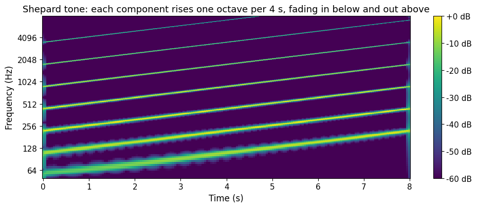
An endlessly rising Shepard tone (8 s):
Risset tones, named after the French composer and scientist Jean-Claude Risset (1938–2016), are often confused with Shepard tones because they are so similar. The difference is that Shepard tones are discrete, while Risset showed the same illusion can be made with continuous sounds, a pitch that seems to rise or fall without end. The effect comes from overlapping sine waves that fade in and out at different frequencies, creating the impression of an endless scale. Risset tones show how our perception of pitch can be steered by careful control of spectral content and amplitude envelopes. The Shepard tones app plays both versions endlessly, rising or falling, stepped or gliding, while drawing the octave components and their amplitude envelope.
Both Shepard and Risset tones have been used in sound design and music. One of many examples is the video Audio Illusion: ascending melody (Advanced Shepard tones) by Smashed Transistors:
Missing fundamental
Another striking auditory illusion is the missing fundamental. When a complex tone lacks its fundamental frequency but keeps its harmonics, listeners still hear the pitch of the missing fundamental. Pitch perception, in other words, is based on the pattern of overtones, not just on the lowest frequency present.
Play a sound with frequencies at 200 Hz, 300 Hz, and 400 Hz (the 2nd, 3rd, and 4th harmonics of 100 Hz) but leave out the 100 Hz fundamental, and most listeners still hear the pitch as if the 100 Hz tone were there. The auditory system reads the spacing between the harmonics and infers the fundamental, even when it is physically absent.
This matters in music and audio technology. Small speakers, like those in smartphones, often cannot reproduce very low frequencies, yet listeners still perceive the intended bass notes from the higher harmonics. The effect is also used in telephony and audio compression to suggest full-range sound from a limited frequency range.
The missing fundamental shows that pitch perception is constructive. The brain detects regularities and patterns in the spectrum rather than simply responding to the frequencies that are physically present. Harmony and melody returns to the same effect under its other name, virtual pitch, and uses it to build melodies out of partials alone.
The figure below shows spectrograms of a complex tone with and without its 100 Hz fundamental, and the two sounds follow. Listen for the pitch staying put while the timbre thins out.
Source
import numpy as np
import librosa
import librosa.display
from IPython.display import Audio, display
import matplotlib.pyplot as plt
plt.rcParams.update({
    "font.size": 10,
    "axes.titlesize": 11,
    "axes.labelsize": 10,
    "xtick.labelsize": 9,
    "ytick.labelsize": 9,
    "legend.fontsize": 9,
    "figure.figsize": (10, 4),
    "figure.dpi": 100,
    "savefig.dpi": 150,
    "axes.spines.top": False,
    "axes.spines.right": False,
})

# The missing fundamental: harmonics 2 to 5 of 100 Hz, with and without the 100 Hz component itself
sr = 22050
f0, dur = 100, 2.0
t = np.linspace(0, dur, int(sr * dur), endpoint=False)
fade = np.minimum(1, np.minimum(t / 0.02, (dur - t) / 0.02))

def complex_tone(harmonics):
    y = sum(np.sin(2 * np.pi * h * f0 * t) / h for h in harmonics)
    return 0.4 * y / np.abs(y).max() * fade

complete = complex_tone([1, 2, 3, 4, 5])
missing = complex_tone([2, 3, 4, 5])

fig, axes = plt.subplots(1, 2, figsize=(10, 3.3), sharey=True)
for ax, y, title in zip(axes, [complete, missing], ['With the 100 Hz fundamental', 'Fundamental removed']):
    S = librosa.amplitude_to_db(np.abs(librosa.stft(y, n_fft=4096)), ref=np.max)
    img = librosa.display.specshow(S, sr=sr, hop_length=1024, x_axis='time', y_axis='log', cmap='viridis', vmin=-60, ax=ax)
    ax.axhline(f0, color='white', linestyle=':', linewidth=1.2)
    ax.set_ylim(50, 1000)
    ax.set_xlabel('Time (s)')
    ax.set_title(title)
axes[0].set_ylabel('Frequency (Hz)')
axes[1].set_ylabel('')
axes[1].text(0.05, f0 * 1.35, 'nothing at 100 Hz,\nyet the pitch is still 100 Hz', color='white')
fig.colorbar(img, ax=axes, format='%+2.0f dB', pad=0.02)
plt.show()

print("Complete tone (100 Hz fundamental plus harmonics):")
display(Audio(complete, rate=sr))
print("The same tone with the 100 Hz fundamental removed: the pitch does not change, only the timbre.")
display(Audio(missing, rate=sr))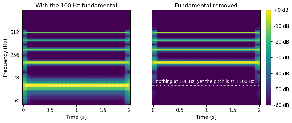
Complete tone (100 Hz fundamental plus harmonics):
The same tone with the 100 Hz fundamental removed: the pitch does not change, only the timbre.
Binaural beats
When two slightly different frequencies are played separately to each ear (using headphones), the listener perceives a rhythmic beating at the frequency difference. This illusion arises from the brain’s processing of phase differences between the ears.
The illusion is best understood next to ordinary beats, which the acoustics chapter introduced. When two tones a few hertz apart are mixed in the same ear, their sum physically swells and fades at the difference frequency, and the beating is there in the waveform for anyone to measure. In the binaural case each ear receives one perfectly steady tone. Nothing in either signal beats. The throbbing arises where the two ears’ signals first meet in the brainstem, in the same circuits that compare timing between the ears for localisation, and it is fainter and softer-edged than the physical kind. The figure below shows the three signals, and the sounds follow; the second one needs headphones.
Source
import numpy as np
from IPython.display import Audio, display
import matplotlib.pyplot as plt
plt.rcParams.update({
    "font.size": 10,
    "axes.titlesize": 11,
    "axes.labelsize": 10,
    "xtick.labelsize": 9,
    "ytick.labelsize": 9,
    "legend.fontsize": 9,
    "figure.figsize": (10, 4),
    "figure.dpi": 100,
    "savefig.dpi": 150,
    "axes.spines.top": False,
    "axes.spines.right": False,
})

# Two tones 6 Hz apart: mixed in one ear they beat physically; one per ear they beat only in the brain
sr = 22050
dur, f1, f2 = 6.0, 400.0, 406.0
t = np.linspace(0, dur, int(sr * dur), endpoint=False)
fade = np.minimum(1, np.minimum(t / 0.05, (dur - t) / 0.05))
a, b = np.sin(2 * np.pi * f1 * t) * fade, np.sin(2 * np.pi * f2 * t) * fade
monaural = 0.2 * (a + b)                       # both tones in both ears: real amplitude beating
binaural = 0.3 * np.vstack([a, b])             # 400 Hz left, 406 Hz right: no beating in the signal

fig, axes = plt.subplots(3, 1, figsize=(10, 5.5), sharex=True)
win = t < 0.5
axes[0].plot(t[win], monaural[win], color='seagreen', linewidth=0.7)
axes[0].set_title('Monaural beats: both tones in the same ear, so the waveform itself swells 6 times a second', loc='left')
axes[1].plot(t[win], binaural[0][win], color='darkorange', linewidth=0.7)
axes[1].set_title('Binaural beats, left ear: a steady 400 Hz tone', loc='left')
axes[2].plot(t[win], binaural[1][win], color='steelblue', linewidth=0.7)
axes[2].set_title('Binaural beats, right ear: a steady 406 Hz tone; the beating exists only in the brain', loc='left')
for ax in axes:
    ax.set_ylim(-0.7, 0.7); ax.set_yticks([]); ax.set_ylabel('Amplitude')
axes[2].set_xlabel('Time (s)')
plt.tight_layout()
plt.show()

print("400 Hz and 406 Hz mixed together in both ears: ordinary beats, audible on loudspeakers too.")
display(Audio(monaural, rate=sr))
print("400 Hz in the left ear and 406 Hz in the right (headphones required): a fainter, throbbing beat that neither ear receives.")
display(Audio(binaural, rate=sr))
print("Control: 400 Hz alone in both ears, no beating.")
display(Audio(0.3 * a, rate=sr))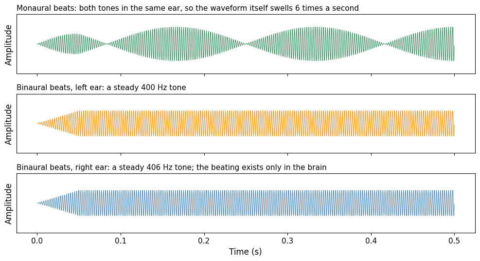
400 Hz and 406 Hz mixed together in both ears: ordinary beats, audible on loudspeakers too.
400 Hz in the left ear and 406 Hz in the right (headphones required): a fainter, throbbing beat that neither ear receives.
Control: 400 Hz alone in both ears, no beating.
A critical look: binaural beats as a brain hack?
Search any streaming service for “binaural beats” and you will find playlists promising focus, deep sleep, or reduced anxiety, each tuned to a specific frequency. The illusion itself is real, as described above. The claims built on top of it deserve a critical look.
- The claim is that the beating percept entrains brain rhythms at the beat frequency, so that a 6 Hz beat induces a relaxed “theta state” and a 40 Hz beat sharpens attention.
- The evidence is a pile of small experiments with mixed results. A meta-analysis of twenty-two studies found a modest average benefit for anxiety, attention, and pain Garcia-Argibay et al., 2019, but the studies differed in beat frequency, duration, masking noise, and outcome measures, and small positive studies reach print more easily than null ones, a problem known as publication bias.
- The method in most studies cannot separate the supposed entrainment from ordinary relaxation, expectation, or simply resting with a steady sound in the ears.
- The limits are therefore sharp. Listening to binaural beats is harmless and may well be pleasant, but the specific frequency-prescription story is not established.
An audible illusion is not evidence of a neural mechanism. That distinction, between what you hear and what it proves, is the core skill this chapter has been practising.
- Fletcher, H., & Munson, W. A. (1933). Loudness, Its Definition, Measurement and Calculation. The Journal of the Acoustical Society of America, 5(2), 82–108. 10.1121/1.1915637
- Bregman, A. S. (1990). Auditory Scene Analysis: The Perceptual Organization of Sound. The MIT Press. 10.7551/mitpress/1486.001.0001
- Gaver, W. W. (1993). What in the World Do We Hear?: An Ecological Approach to Auditory Event Perception. Ecological Psychology, 5(1), 1–29. 10.1207/s15326969eco0501_1
- Clarke, E. F. (2005). Ways of Listening: An Ecological Approach to the Perception of Musical Meaning. Oxford University Press. 10.1093/acprof:oso/9780195151947.001.0001
- Jensenius, A. R. (2022). Sound Actions: Conceptualizing Musical Instruments. The MIT Press. 10.7551/mitpress/14220.001.0001
- Fastl, H., & Zwicker, E. (2007). Psychoacoustics. Springer Berlin Heidelberg. 10.1007/978-3-540-68888-4
- Shepard, R. N. (1964). Circularity in Judgments of Relative Pitch. The Journal of the Acoustical Society of America, 36(12), 2346–2353. 10.1121/1.1919362
- Garcia-Argibay, M., Santed, M. A., & Reales, J. M. (2019). Efficacy of Binaural Auditory Beats in Cognition, Anxiety, and Pain Perception: A Meta-Analysis. Psychological Research, 83(2), 357–372. 10.1007/s00426-018-1066-8
- Moore, B. (1997). An Introduction to the Psychology of Hearing: Fourth Edition. BRILL. 10.1163/9789004658820
- Cook, P. R. (Ed.). (1999). Music, Cognition, and Computerized Sound: An Introduction to Psychoacoustics. The MIT Press. 10.7551/mitpress/4808.001.0001