Earlier units on acoustics and psychoacoustics introduced frequency, spectrum, and pitch perception. This chapter reconnects those ideas to note names, intervals, scales, and chords, working between perception and interpretation in the four levels of description: a pitch is heard, but a tonic, a cadence, and a deceptive resolution are cultural categories laid over what is heard.
Tones
The chapter looks at how frequencies interact both horizontally and vertically. Horizontal organisation gives rise to melodies: sequences of pitches unfolding over time, often shaped by rhythmic patterns. Vertical organisation produces intervals, harmonies, and textures, as several pitches sound together or overlap. First, though, we need to define the tone.
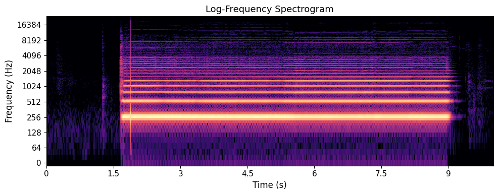
In music theory and psychology, a tone is a sound with a specific frequency, timbral quality, and temporal shape that the auditory system interprets as having a definite pitch. How we perceive tones depends both on the physical properties of the sound wave (frequency, amplitude, and harmonic content) and on the way our brains process these signals. Tones are the building blocks of music perception, letting us distinguish melodies, harmonies, and textures.
Tones can be generated, analysed, and manipulated with digital tools. Synthesisers build them by combining waveforms, while audio analysis software extracts pitch and timbre features from recordings. Pitch detection algorithms and spectral analysis underpin music information retrieval, automatic transcription, and digital instrument design.
Source
import librosa
import librosa.display
import numpy as np
import IPython.display as ipd
import matplotlib.pyplot as plt
plt.rcParams.update({
    "font.size": 10,
    "axes.titlesize": 11,
    "axes.labelsize": 10,
    "xtick.labelsize": 9,
    "ytick.labelsize": 9,
    "legend.fontsize": 9,
    "figure.figsize": (10, 4),
    "figure.dpi": 100,
    "savefig.dpi": 150,
    "axes.spines.top": False,
    "axes.spines.right": False,
})

audio_path = "audio/SoundAction122-Saxophone_tone.wav"
y, sr = librosa.load(audio_path, sr=None)

S = librosa.stft(y)
S_db = librosa.amplitude_to_db(abs(S), ref=np.max)

plt.figure(figsize=(10, 4))
librosa.display.specshow(S_db, sr=sr, x_axis='time', y_axis='log')
plt.title('Log-Frequency Spectrogram')
plt.xlabel("Time (s)")
plt.ylabel("Frequency (Hz)")
plt.tight_layout()
plt.show()

ipd.Audio(y, rate=sr)
Pitch
Pitch is the psycho-physiological correlate of frequency that lets us hear one sound as higher or lower than another. It is closely related to the fundamental frequency of a tone, but the relationship is not one-to-one. As you may recall from the acoustics chapter, most instrument tones are not pure sine waves. Musical, “pitched” instruments generally produce a fundamental frequency (often abbreviated f0), which defines the perceived pitch. Additional overtones define the timbre of the instrument. Many musical instruments have overtones that are in a “harmonic” relationship to the fundamental frequency (f1, f2, etc.). For a tone with a fundamental frequency of 220 Hz, the harmonic overtones—sometimes called partials—are 440 Hz, 660 Hz, 880 Hz, etc. The individual partials of a complex sound are typically not heard as separate; our perceptual system fuses them into a single sound.
The pitch of harmonic tones generally corresponds to the fundamental frequency (f0). However, the brain can infer a fundamental frequency (and thus perceive pitch) from complex tones even when a fundamental component is absent. This is the missing fundamental you met in psychoacoustics, where it appeared as evidence that pitch perception is constructive. In a musical context it usually goes by its other name, virtual pitch, and the demonstrations below put it to work: with the right partials and no fundamental at all, you will hear a melody that is not physically in the signal.
Below is a sequence of simple (sine) tones at different frequencies.
Source
import librosa

import librosa.display
import matplotlib.pyplot as plt
plt.rcParams.update({
    "font.size": 10,
    "axes.titlesize": 11,
    "axes.labelsize": 10,
    "xtick.labelsize": 9,
    "ytick.labelsize": 9,
    "legend.fontsize": 9,
    "figure.figsize": (10, 4),
    "figure.dpi": 100,
    "savefig.dpi": 150,
    "axes.spines.top": False,
    "axes.spines.right": False,
})

y_tones, sr_tones = librosa.load("audio/week7_tones1.mp3", sr=None)
S_tones = librosa.stft(y_tones)
S_tones_db = librosa.amplitude_to_db(abs(S_tones), ref=np.max)

plt.figure(figsize=(10, 4))
librosa.display.specshow(S_tones_db, sr=sr_tones, x_axis='time', y_axis='log')
plt.title('Log-Frequency Spectrogram')
plt.xlabel("Time (s)")
plt.ylabel("Frequency (Hz)")
plt.tight_layout()
plt.show()

import IPython.display as ipd

ipd.Audio(y_tones, rate=sr_tones)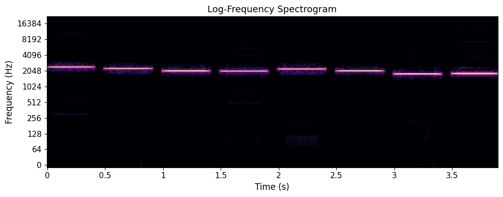
If we add some partials (multiples) below each tone, can you start to hear a familiar melody?
Source
import librosa

import librosa.display
import matplotlib.pyplot as plt
plt.rcParams.update({
    "font.size": 10,
    "axes.titlesize": 11,
    "axes.labelsize": 10,
    "xtick.labelsize": 9,
    "ytick.labelsize": 9,
    "legend.fontsize": 9,
    "figure.figsize": (10, 4),
    "figure.dpi": 100,
    "savefig.dpi": 150,
    "axes.spines.top": False,
    "axes.spines.right": False,
})

y_tones, sr_tones = librosa.load("audio/week7_tones2.mp3", sr=None)
S_tones = librosa.stft(y_tones)
S_tones_db = librosa.amplitude_to_db(abs(S_tones), ref=np.max)

plt.figure(figsize=(10, 4))
librosa.display.specshow(S_tones_db, sr=sr_tones, x_axis='time', y_axis='log')
plt.title('Log-Frequency Spectrogram')
plt.xlabel("Time (s)")
plt.ylabel("Frequency (Hz)")
plt.tight_layout()
plt.show()

import IPython.display as ipd

ipd.Audio(y_tones, rate=sr_tones)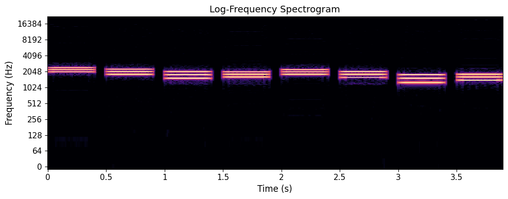
If we then rearrange these partials slightly, we can induce an even stronger sense of virtual pitch, that is, various missing fundamental frequencies which are not physically present in the tones themselves:
Source
import librosa

import librosa.display
import matplotlib.pyplot as plt
plt.rcParams.update({
    "font.size": 10,
    "axes.titlesize": 11,
    "axes.labelsize": 10,
    "xtick.labelsize": 9,
    "ytick.labelsize": 9,
    "legend.fontsize": 9,
    "figure.figsize": (10, 4),
    "figure.dpi": 100,
    "savefig.dpi": 150,
    "axes.spines.top": False,
    "axes.spines.right": False,
})

y_tones, sr_tones = librosa.load("audio/week7_tones3.mp3", sr=None)
S_tones = librosa.stft(y_tones)
S_tones_db = librosa.amplitude_to_db(abs(S_tones), ref=np.max)

plt.figure(figsize=(10, 4))
librosa.display.specshow(S_tones_db, sr=sr_tones, x_axis='time', y_axis='log')
plt.title('Log-Frequency Spectrogram')
plt.xlabel("Time (s)")
plt.ylabel("Frequency (Hz)")
plt.tight_layout()
plt.show()

import IPython.display as ipd

ipd.Audio(y_tones, rate=sr_tones)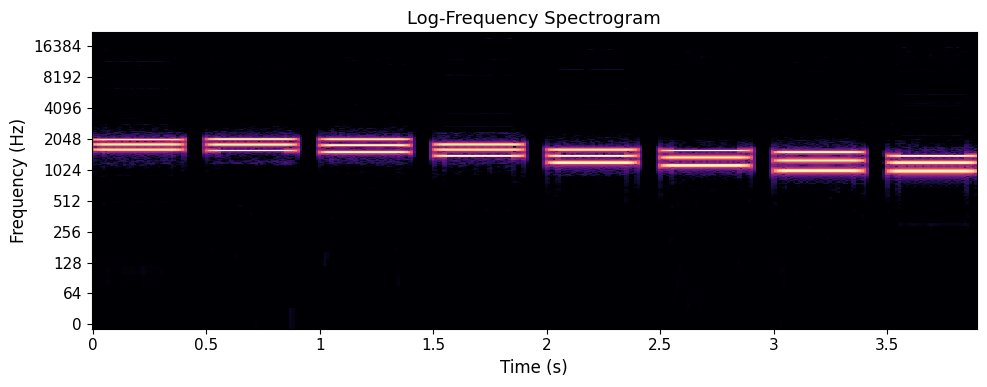
What happens is that your brain creates a virtual fundamental based on “calculating” the underlying frequencies part of the harmonic series.
Source
import numpy as np
import matplotlib.pyplot as plt
plt.rcParams.update({
    "font.size": 10,
    "axes.titlesize": 11,
    "axes.labelsize": 10,
    "xtick.labelsize": 9,
    "ytick.labelsize": 9,
    "legend.fontsize": 9,
    "figure.figsize": (10, 4),
    "figure.dpi": 100,
    "savefig.dpi": 150,
    "axes.spines.top": False,
    "axes.spines.right": False,
})

# Each half-second segment: three partials, chosen so that they are consecutive
# harmonics of a fundamental that is not itself present.
segments = [
    (200, [8, 9, 10]), (225, [7, 8, 9]), (250, [6, 7, 8]), (200, [7, 8, 9]),
    (200, [6, 7, 8]), (225, [5, 6, 7]), (250, [4, 5, 6]), (200, [5, 6, 7]),
]
seg = 0.5

fig, ax = plt.subplots(figsize=(10, 4.2))
for k, (f0, harmonics) in enumerate(segments):
    t0, t1 = k * seg + 0.02, (k + 1) * seg - 0.02
    for h in harmonics:
        ax.hlines(f0 * h, t0, t1, color="steelblue", linewidth=3)
    ax.hlines(f0, t0, t1, color="firebrick", linewidth=3)
    if k == 0:
        for h in range(1, harmonics[0]):
            ax.hlines(f0 * h, t0, t1, color="0.6", linestyle=":", linewidth=1)
ax.annotate("1600, 1800, 2000 Hz\nare harmonics 8, 9, 10\nof 200 Hz", xy=(0.25, 2000), xytext=(1.0, 2350),
            color="0.3", arrowprops=dict(arrowstyle="->", color="0.5"))
ax.text(0.55, 800, "harmonics 1 to 7\nare absent", ha="left", va="center", color="0.5", fontsize=9)
ax.text(4.05, 2000, "spectral pitches\n(what is in the signal)", va="center", color="steelblue")
ax.text(4.05, 220, "virtual pitch\n(what you hear)", va="center", color="firebrick")
ax.set_xlim(0, 5.1)
ax.set_ylim(0, 3000)
ax.set_xlabel("Time (s)")
ax.set_ylabel("Frequency (Hz)")
ax.set_title("Virtual pitch: three high partials imply a fundamental that is not in the signal")
ax.grid(alpha=0.3)
plt.tight_layout()
plt.show()
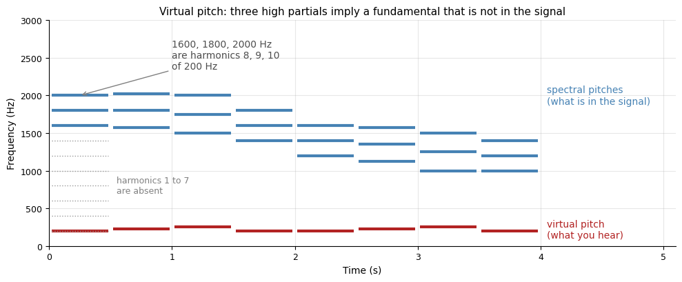
Figure: Eight short tones, each made of three partials (blue). The brain finds the fundamental they share (red) and hears that as the pitch, so the melody moves even though no partial follows it. Schematic, after lecture materials by Petri Toiviainen (2015).
Constant-Q transform
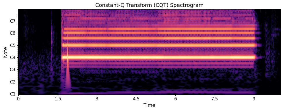
So far we have looked at regular spectrograms, both linear and logarithmic. Each has its uses, but the logarithmic version represents human hearing more closely. For pitch, the constant-Q transform (CQT) works better still, since it maps frequencies to musical notes. Where the standard spectrogram uses a linear frequency scale, the CQT uses a logarithmic one that matches how notes are spaced, with each octave divided into equal steps. This makes it easier to see which pitch classes are present, which suits tasks like chord recognition, key detection, and melody analysis.
Real musical notes are not pure, since they carry overtones and partials that are not perfectly harmonic. In a CQT spectrogram, this shows up as energy spread across several frequency bins rather than sitting only at the fundamental. We can therefore see both the main pitches and their harmonic content, which tells us about the timbre and structure of the sound.
Source
import librosa
import librosa.display
import numpy as np
import IPython.display as ipd
import matplotlib.pyplot as plt
plt.rcParams.update({
    "font.size": 10,
    "axes.titlesize": 11,
    "axes.labelsize": 10,
    "xtick.labelsize": 9,
    "ytick.labelsize": 9,
    "legend.fontsize": 9,
    "figure.figsize": (10, 4),
    "figure.dpi": 100,
    "savefig.dpi": 150,
    "axes.spines.top": False,
    "axes.spines.right": False,
})

audio_path = "audio/SoundAction122-Saxophone_tone.wav"
y, sr = librosa.load(audio_path, sr=None)
C = librosa.cqt(y, sr=sr)
C_db = librosa.amplitude_to_db(np.abs(C), ref=np.max)

plt.figure(figsize=(10, 4))
librosa.display.specshow(C_db, sr=sr, x_axis='time', y_axis='cqt_note')
plt.title('Constant-Q Transform (CQT) Spectrogram')
plt.tight_layout()
plt.show()

ipd.Audio(y, rate=sr)
Pitch class
In music, a pitch class is a set of pitches that are a whole number of octaves apart, e.g., the pitch class C consists of the Cs in all octaves. Humans perceive the notes in a tonal scale as repeating once per octave. This provides the basis for producing and perceiving melodic patterns based on relative pitch relationships, that is, relative to a pitch class. Absolute pitch ability, on the other hand, is the ability to recognise (or reproduce) specific pitches without the help of a reference pitch and pitch class.
Source
import numpy as np
import matplotlib.pyplot as plt
plt.rcParams.update({
    "font.size": 10,
    "axes.titlesize": 11,
    "axes.labelsize": 10,
    "xtick.labelsize": 9,
    "ytick.labelsize": 9,
    "legend.fontsize": 9,
    "figure.figsize": (10, 4),
    "figure.dpi": 100,
    "savefig.dpi": 150,
    "axes.spines.top": False,
    "axes.spines.right": False,
})

from mpl_toolkits.mplot3d import Axes3D  # noqa: F401  (registers the 3d projection)

names = ["C", "C#", "D", "D#", "E", "F", "F#", "G", "G#", "A", "A#", "B"]
octaves = 2.5
theta = np.linspace(0, 2 * np.pi * octaves, 600)
x, y, z = np.cos(theta), np.sin(theta), theta / (2 * np.pi)

fig = plt.figure(figsize=(10, 5.2))
ax = fig.add_subplot(projection="3d")
ax.plot(x, y, z, color="steelblue", linewidth=2.5)
ax.plot(np.cos(theta[:600 // 5 * 2]), np.sin(theta[:600 // 5 * 2]), np.zeros(240), color="0.8", linewidth=1)
for k, name in enumerate(names):                                   # chroma labels round the base
    a = 2 * np.pi * k / 12
    ax.text(1.18 * np.cos(a), 1.18 * np.sin(a), 0, name, ha="center", va="center", color="0.3")
for octave in range(3):                                            # the Cs stack vertically
    ax.scatter([1], [0], [octave], color="firebrick", s=40, zorder=5)
    ax.text(1.0, 0.32, octave + 0.12, f"C{octave + 3}", color="firebrick")
ax.plot([1, 1], [0, 0], [0, 2], color="firebrick", linestyle="--", linewidth=1)
ax.plot([0, 0], [0, 0], [0, octaves + 0.3], color="0.4", linewidth=1)
ax.text(0, 0, octaves + 0.45, "pitch height", ha="center", color="0.4")
ax.text(0, -1.5, -0.35, "chroma (pitch class)", ha="center", color="0.4")
ax.set_axis_off()
ax.view_init(elev=22, azim=-60)
ax.set_box_aspect((1, 1, 1.3))
plt.title("The pitch helix: height rises continuously while chroma repeats every octave")
plt.tight_layout()
plt.show()
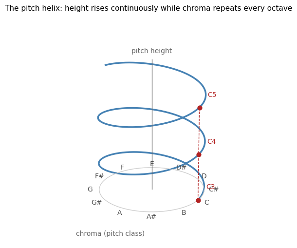
Figure: Going up the helix, pitch height increases steadily, but every full turn returns to the same chroma, so all the Cs lie on one vertical line. After Shepard (1964).
Chromagram
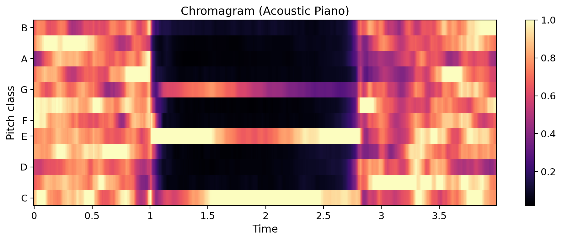
A chromagram visualises the intensity of each of the 12 pitch classes (C, C#, D, ..., B) over time, regardless of octave. Below is a chromagram of the saxophone tone used above. Notice how the algorithm is less certain during the noisy attack and release portions, but clearly identifies the main pitch (C) during the sustained part of the tone. The presence of energy in the fifth (G) and third (E) pitch classes reflects their harmonic relationship to the tonic (C). Chromagrams are useful for analysing harmonic and melodic content in music, as they abstract away octave information and focus on pitch class structure.
Source
import matplotlib.pyplot as plt
plt.rcParams.update({
    "font.size": 10,
    "axes.titlesize": 11,
    "axes.labelsize": 10,
    "xtick.labelsize": 9,
    "ytick.labelsize": 9,
    "legend.fontsize": 9,
    "figure.figsize": (10, 4),
    "figure.dpi": 100,
    "savefig.dpi": 150,
    "axes.spines.top": False,
    "axes.spines.right": False,
})
chroma = librosa.feature.chroma_cqt(y=y, sr=sr)
plt.figure(figsize=(10, 4))
librosa.display.specshow(chroma, x_axis='time', y_axis='chroma', sr=sr)
plt.colorbar()
plt.title('Chromagram (Chroma CQT)')
plt.tight_layout()
plt.show()

ipd.Audio(y, rate=sr)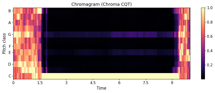
Scales and tonality
Scales and modes
A scale is the set of pitch classes a piece of music draws on, listed in ascending order within one octave. Most Western music since around 1600 uses the major and minor scales, seven-note scales built from a fixed pattern of whole steps (W) and half steps (H): W W H W W W H for major. Starting the same pattern from a different note gives the modes (Dorian, Mixolydian, and so on) familiar from folk, jazz, and film music. Pentatonic (five-note) scales, such as the black keys on a piano, turn up in an astonishing number of traditions worldwide. One likely reason is perceptual: with only five notes there are no semitone clashes, so almost any two notes sound acceptable together.
On a piano the octave is divided into 12 equal semitones, a system called 12-tone equal temperament (12-TET). Each semitone multiplies the frequency by the twelfth root of two, about 1.0595. For finer measurement, a semitone is split into 100 cents, so an octave is 1200 cents. Cents matter because the ear is sensitive to differences far smaller than a semitone: trained listeners can hear a few cents of mistuning in a sustained chord, and the piano’s major third is 14 cents wider than the pure 5:4 third of the harmonic series. You will hear that difference in the Harmony section below.
Dig deeper: cents and pure intervals
The number of cents between two frequencies is
so a frequency ratio of 2:1 gives 1200 cents and each equal-tempered semitone is exactly 100. The table compares the pure ratios found in the harmonic series with their equal-tempered approximations.
| Interval | Pure ratio | Pure (cents) | 12-TET (cents) | Difference |
|---|---|---|---|---|
| Octave | 2:1 | 1200 | 1200 | 0 |
| Perfect fifth | 3:2 | 702 | 700 | 2 |
| Perfect fourth | 4:3 | 498 | 500 | 2 |
| Major third | 5:4 | 386 | 400 | 14 |
| Minor third | 6:5 | 316 | 300 | 16 |
Fifths and fourths survive equal temperament almost intact; thirds do not, which is why the equal-tempered third beats audibly against a pure one. Historical temperaments (meantone, well temperament) were different compromises over where to put this error.
We number the notes of a scale from the tonic as scale degrees 1 to 7, and use Roman numerals for chords built on those degrees. The figure below shows a short melody that walks up and down the C major scale and comes to rest on a whole note.

Figure: A melody up and down the C major scale, eighth notes in the first bar and a whole note on the tonic in the second.
The Scale explorer app lets you build any scale on any tonic, from the major scale and the modes to pentatonic, blues, and whole-tone scales, and hear it over a drone. It draws the scale on a pitch-class circle and on a keyboard, lists each degree’s distance from the tonic in semitones and cents, and switches between equal temperament and just intonation, so the beating third of the table above can be heard locking into place.
Tonality and harmonic expectation
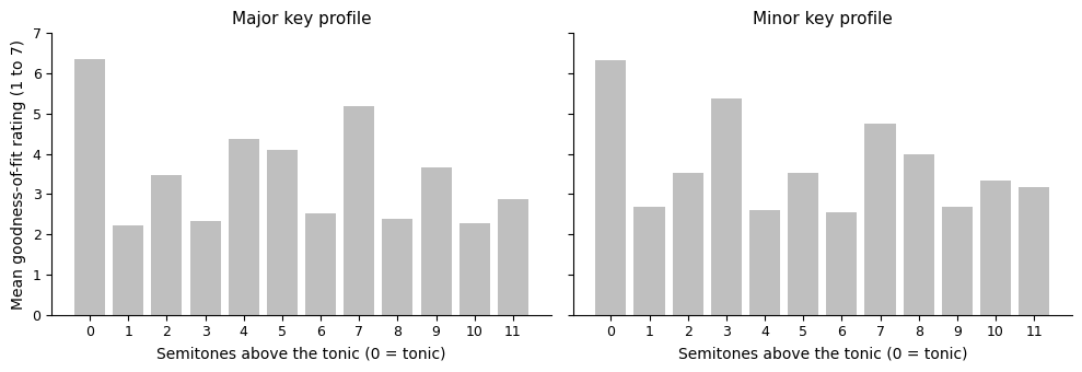
Tonality is the organisation of pitches and chords around a central note called the tonic, creating a sense of hierarchy and resolution in music. In Western music, tonality underlies the concept of key signatures (e.g., “C major”, “A minor”), where certain notes and chords feel stable (restful) while others create tension and seek resolution. This hierarchy is learned implicitly through exposure to music, forming a cognitive schema that shapes our expectations of which notes or chords will follow. Krumhansl (2001) measured these hierarchies experimentally, and the resulting tonal profiles are still the basis of most computational key-finding, including the estimate you will meet in machine listening. Tonality is also supported by acoustics. The most important notes in a scale, such as the third and fifth, share harmonic overtones with the tonic, reinforcing their sense of belonging. Even without formal music theory training, listeners develop an intuitive sense of tonality and harmonic expectation through cultural experience.
Krumhansl (2001) measured the hierarchy with the probe-tone method. Listeners hear a short passage that establishes a key, such as a scale or a cadence, followed by a single “probe” tone, and rate how well the probe fits what came before. Averaged over many listeners, the ratings form a key profile: the tonic fits best, then the fifth and the third, then the remaining notes of the scale, and the five notes outside the scale fit worst. The plot below shows the profiles for major and minor keys. Notice that the profile is not simply “in the scale or not”: the scale notes themselves form a hierarchy, and that hierarchy is what a melody plays with when it builds and releases tension.
Source
import numpy as np
import matplotlib.pyplot as plt
plt.rcParams.update({
    "font.size": 10,
    "axes.titlesize": 11,
    "axes.labelsize": 10,
    "xtick.labelsize": 9,
    "ytick.labelsize": 9,
    "legend.fontsize": 9,
    "figure.figsize": (10, 4),
    "figure.dpi": 100,
    "savefig.dpi": 150,
    "axes.spines.top": False,
    "axes.spines.right": False,
})

# Krumhansl and Kessler (1982) probe-tone ratings, averaged over listeners
pcs = [str(s) for s in range(12)]
major = [6.35, 2.23, 3.48, 2.33, 4.38, 4.09, 2.52, 5.19, 2.39, 3.66, 2.29, 2.88]
minor = [6.33, 2.68, 3.52, 5.38, 2.60, 3.53, 2.54, 4.75, 3.98, 2.69, 3.34, 3.17]

fig, axes = plt.subplots(1, 2, figsize=(10, 3.5), sharey=True)
for ax, profile, name in zip(axes, [major, minor], ["Major key", "Minor key"]):
    ax.bar(pcs, profile, color="0.75")
    ax.set_title(f"{name} profile")
    ax.set_xlabel("Semitones above the tonic (0 = tonic)")
    ax.set_ylim(0, 7)
axes[0].set_ylabel("Mean goodness-of-fit rating (1 to 7)")
plt.tight_layout()
plt.show()
Cultural frames beyond Western tonality
The concepts in this chapter are often introduced through Western tonal theory, but melody and harmony are organised differently across musical cultures. Some traditions use scales and intonation systems that do not map neatly onto 12-tone equal temperament, while others prioritise melodic motion, ornamentation, drone relationships, or modal centres over functional chord progressions.
Examples include microtonal pitch systems, raga-based melodic organisation, maqam traditions with characteristic intonation and melodic pathways, and ensemble practices where heterophony is central. These approaches show that harmony and melody are not universal rule sets but culturally shaped listening and performance practices. In Karnatak vocal lessons, for example, much of a raga’s melodic shape is carried by the teacher’s hands as well as the voice Pearson, 2013.
Analysis tools are theory-dependent. If we only use Western note grids and chord labels, we may miss musically important details in other repertoires.
Scales invented in the twentieth century push the point further: some of them abandon the octave itself. The example below lets you hear the timbre effect. It plays an ascending Bohlen-Pierce scale and a 3:5:7 chord twice: first with an odd-harmonic timbre that matches the scale, then with a full harmonic timbre that does not.
Source
import numpy as np
from IPython.display import Audio, display

sr = 22050
t_note = np.linspace(0, 0.4, int(sr * 0.4), endpoint=False)
t_chord = np.linspace(0, 3.0, int(sr * 3.0), endpoint=False)

def tone(f, t, harmonics):
    """Sum of partials with 1/h amplitudes and a short fade at each end."""
    y = sum((1.0 / h) * np.sin(2 * np.pi * f * h * t) for h in harmonics)
    fade = int(0.02 * sr)
    env = np.ones_like(t)
    env[:fade] = np.linspace(0, 1, fade)
    env[-fade:] = np.linspace(1, 0, fade)
    return y * env

odd = range(1, 10, 2)        # 1, 3, 5, 7, 9: clarinet-like
full = range(1, 10)          # 1 to 9: all harmonics

root = 220.0
tritave = 3.0
bp_steps = [root * tritave ** (k / 13) for k in range(14)]  # 13 steps plus the tritave
bp_chord = [root, root * 5 / 3, root * 7 / 3]               # the 3:5:7 "triad"

for label, harmonics in [("odd harmonics (matched)", odd), ("all harmonics (mismatched)", full)]:
    scale = np.concatenate([tone(f, t_note, harmonics) for f in bp_steps])
    chord = sum(tone(f, t_chord, harmonics) for f in bp_chord)
    print(f"Bohlen-Pierce scale, {label}:")
    display(Audio(0.2 * scale / np.max(np.abs(scale)), rate=sr))
    print(f"3:5:7 chord, {label}:")
    display(Audio(0.2 * chord / np.max(np.abs(chord)), rate=sr))
Bohlen-Pierce scale, odd harmonics (matched):
3:5:7 chord, odd harmonics (matched):
Bohlen-Pierce scale, all harmonics (mismatched):
3:5:7 chord, all harmonics (mismatched):
Dig deeper: scales that are not built on the octave
Twelve-tone equal temperament makes two choices that are easy to mistake for laws of nature: the scale repeats at the octave (2:1), and the octave is cut into twelve equal steps. Neither is forced. Loosening them gives a family of non-traditional scales, each of which tells us something about how pitch and consonance work.
Bohlen-Pierce. The best-known octave-free scale divides the tritave, the 3:1 interval of a perfect twelfth, into 13 equal steps of about 146 cents. It was found independently three times, by the engineer Heinz Bohlen in 1972, by Kees van Prooijen in 1978, and by John Pierce in 1984. Its steps closely approximate ratios built from the odd numbers 3, 5, and 7, so the scale has its own “triad”, the chord 3:5:7, which plays the role that 4:5:6 plays for the major triad. The catch is timbre. A tone with all harmonics contains the octave (2:1) in its own spectrum, so an octave-free scale clashes with it. With tones made of odd harmonics only, such as a clarinet in its low register or a square-like synthesised tone, the partials of the 3:5:7 chord line up and the scale locks into place. Mathews et al. (1988) tested this at Bell Labs: listeners rated Bohlen-Pierce chords for consonance much as they rate ordinary triads, once the timbre matched. Clarinets have since been built with Bohlen-Pierce keywork, and there is a small but active repertoire.
Other equal divisions of the octave. Keeping the octave but changing the number of steps gives 19, 31, or 53 equal divisions (written 19-EDO and so on). 31-EDO, championed by Christiaan Huygens, is almost identical to the quarter-comma meantone temperament of Renaissance keyboards and has excellent major thirds. 53-EDO contains near-perfect fifths and thirds and was known to Chinese and European theorists centuries ago. These scales keep familiar harmony intact but make the “cracks” of 12-tone tuning audible, because each has a different set of intervals that it gets right.
Just intonation. Harry Partch went in the opposite direction and abandoned equal steps altogether, building a 43-tone scale of pure ratios up to the 11th harmonic and a set of instruments to play it. Just systems give beat-free chords in some keys and unusable ones in others, which is the trade-off that temperaments were invented to manage.
Non-octave equal steps. Wendy Carlos’s alpha, beta, and gamma scales (steps of about 78, 64, and 35 cents) stack a single small interval that never lands on an octave at all, yet approximate pure fifths and thirds very closely. The result is music with recognisable harmony but no octave equivalence, so a melody transposed “up an octave” ends up on different scale degrees.
Why this matters for perception. Sethares (2005) argues that consonance is not a property of an interval alone but of the pairing between a scale and a spectrum. A timbre with harmonic partials favours the octave and the fifth. Retune the partials and different intervals become smooth, which is exactly what the Bohlen-Pierce experiments showed. Non-traditional scales are therefore natural test cases for the question that runs through this chapter: how much of what we hear as consonant is acoustics, how much is timbre, and how much is what we grew up hearing?
Statistical learning, expectation, and enculturation
Harmonic and melodic listening rely on implicit knowledge of regularities in the music you have heard, which is often studied under statistical learning and implicit harmony. Enculturated listeners internalise probabilities (which chord tends to follow which, typical melodic skips vs steps) that shape expectation and surprise. Huron (2006) builds a general theory of musical affect on exactly this mechanism, and Margulis (2018) is a short, accessible way in. Those expectations are culture-relative, since competence in one grammar does not transfer wholesale to another.
When you analyse scores or audio, separate three layers:
- Acoustic facts (intervals, spectra, roughness),
- Style-specific syntax (voice-leading norms, modal centres, idiomatic ornament),
- Analytic vocabulary (Roman numerals, chord labels, computer features), where each tool reveals some things and hides others.
Cross-traditional comparison should name the tool’s assumptions, as the previous section argued.
Harmony
Harmony is the simultaneous sounding of different pitches, combined into intervals and chords and shaped by timbre and texture. These combinations carry much of the emotional tone and complexity of a piece, and they can evoke a wide range of responses in the listener.
Intervals
An interval is the distance between two pitches, measured in steps or frequency ratios. Intervals are the building blocks of harmony, as they define the relationships between notes played together or in succession. In Western music theory, intervals are named by counting the number of letter names from the lower to the higher note (e.g., C to E is a third). They can be major, minor, perfect, augmented, or diminished.
The human brain is sensitive to the relationships between pitches, perceiving certain combinations as consonant (pleasant or stable) and others as dissonant (tense or unstable). For example, some intervals, like octaves and perfect fifths, are perceived as consonant, while others, like minor seconds or tritones, are more dissonant. These perceptual responses are influenced by cultural exposure, musical training, and innate auditory processing mechanisms. In the Interval lab app you can play any interval with two complex tones, compare just intonation with equal temperament, and rank intervals by consonance against typical listener ratings.
Intervals form the basis for chords and harmonic progressions. The combination of intervals within a chord determines its character and function. A just major third is the simple ratio 5:4; the equal-tempered third used on a piano is slightly wider (the twelfth root of two, to the fourth power). When you sound the two notes together, the just third locks; the equal-tempered one beats gently as nearby harmonics drift in and out of phase.
Source
import numpy as np
from IPython.display import Audio, display

sr = 22050
dur = 3.0
t = np.linspace(0, dur, int(sr * dur), endpoint=False)

def tone(f):
    return sum((1.0 / h) * np.sin(2 * np.pi * f * h * t) for h in range(1, 6))

root = 261.63                       # C4
just = 0.1 * (tone(root) + tone(root * 5 / 4))
equal = 0.1 * (tone(root) + tone(root * 2 ** (4 / 12)))

print("Major third, just intonation (5:4) - stable:")
display(Audio(just, rate=sr))
print(f"Major third, equal temperament ({2 ** (4/12):.4f}:1) - gentle beating:")
display(Audio(equal, rate=sr))
Major third, just intonation (5:4) - stable:
Major third, equal temperament (1.2599:1) - gentle beating:

Figure: The thirteen intervals from unison to octave above C: perfect unison (P1), minor and major second (m2, M2), minor and major third (m3, M3), perfect fourth (P4), augmented fourth or tritone (A4), perfect fifth (P5), minor and major sixth (m6, M6), minor and major seventh (m7, M7), and perfect octave (P8).
Chords
A chord is a group of three or more notes played simultaneously. Chords are the foundation of Western harmony and are used to create progressions that define the structure and mood of a piece.
Triads are the most basic chords, consisting of three notes (root, third, fifth). Types include major, minor, diminished, and augmented triads.

Figure: The four triads on C: major, minor, diminished, and augmented, with their chord symbols above and names below.
More complex chords can be created by adding additional notes, such as sevenths, ninths, elevenths, and thirteenths, which creates richer harmonies.

Figure: Extended chords on C: the seventh, ninth, eleventh, and thirteenth, each adding a third on top of the last.
When combined, chords create progressions that produce movement and tension-resolution patterns. Chords are labelled with Roman numerals after the scale degree of their root, upper case for major and lower case for minor: in C major, I is C major, ii is D minor, IV is F major, and V is G major. Two of the most common progressions are I–IV–V–I in classical and popular music and ii–V–I in jazz. In functional analysis, chords are defined by their roles (tonic, dominant, subdominant) and guide the listener’s expectations.

Figure: The I–IV–V–I progression in C major, with chord symbols above and Roman numerals below.

Figure: The ii–V–I progression in C major, with the tonic first: I, ii, V, I.
Voice leading: connecting harmony and melody
Voice leading describes how individual melodic lines move from one chord to the next. It links vertical harmony (what notes sound together) to horizontal melody (how lines unfold over time).
Good voice leading often aims for:
- Stepwise motion: move by small intervals where possible.
- Common-tone retention: keep shared notes in place between chords.
- Balanced independence: each line has a clear contour without excessive leaps.
- Controlled parallels: in many styles, consecutive parallel perfect fifths or octaves are avoided to preserve line independence.
When these principles are applied, chord progressions tend to sound smoother and more coherent.
Cadences: patterns of tension and release
A cadence is a harmonic-melodic pattern that signals a point of arrival, pause, or continuation.
Common cadence types in tonal music include:
- Authentic cadence (V-I): strongest sense of closure.
- Half cadence (...-V): ends on dominant, creating expectation.
- Plagal cadence (IV-I): softer resolution.
- Deceptive cadence (V-vi): expected resolution is delayed or redirected.
Cadences are heard through melodic behaviour, timing, articulation, and timbre, not only through chord labels. The same cadence can feel final, weak, or ambiguous depending on performance context.
The Chord lab app lets you build any of these chords on any root, in any inversion and voicing, and hear and see it on a keyboard and a staff, and then string chords into a progression in a chosen key: the presets include I–IV–V–I, ii–V–I, and the four cadence types. It chooses voicings that move each voice as little as possible and draws the voice-leading lines, and a live chromagram with a running key estimate shows the chapter’s key-finding idea working on your own progression.
Harmonic rhythm
Harmony also has a rhythm. The rate at which chords change, the harmonic rhythm, is one of the places where this chapter meets time and rhythm. In most tonal music chords change on strong beats, cadences arrive on the downbeat of a bar, and the harmonic rhythm often slows towards a phrase ending. Change the chord on a weak beat, or hold one chord across a bar line, and the same progression feels syncopated or suspended. Listeners use these regularities the same way they use metre: a chord change is expected at certain moments, and a change that comes early or late is heard as an event in itself.
Studying music theory through psychology and technology is revealing because the idealised concepts of Western art music rarely exist in real life. Even a simple triad on an acoustic piano carries considerable timbral complexity, as you can both hear and see below. Real sounds are shaped by the instrument’s physical properties, the performer’s nuances, and the acoustic environment, producing overtones and spectral features that go well beyond the abstract “perfect” chords of theory. To understand how musical structures are actually perceived, we need to analyse real audio signals.
Source
import librosa

import librosa.display
import matplotlib.pyplot as plt
plt.rcParams.update({
    "font.size": 10,
    "axes.titlesize": 11,
    "axes.labelsize": 10,
    "xtick.labelsize": 9,
    "ytick.labelsize": 9,
    "legend.fontsize": 9,
    "figure.figsize": (10, 4),
    "figure.dpi": 100,
    "savefig.dpi": 150,
    "axes.spines.top": False,
    "axes.spines.right": False,
})

# Load the audio file
y_piano, sr_piano = librosa.load("audio/SoundAction074-Acoustic_piano.wav", sr=None)

# CQT Spectrogram
C_piano = librosa.cqt(y_piano, sr=sr_piano)
C_piano_db = librosa.amplitude_to_db(abs(C_piano), ref=np.max)

plt.figure(figsize=(10, 4))
librosa.display.specshow(C_piano_db, sr=sr_piano, x_axis='time', y_axis='cqt_note')
plt.colorbar(format='%+2.0f dB')
plt.title('CQT Spectrogram (Acoustic Piano)')
plt.tight_layout()
plt.show()

# Chromagram
chroma_piano = librosa.feature.chroma_cqt(y=y_piano, sr=sr_piano)
plt.figure(figsize=(10, 4))
librosa.display.specshow(chroma_piano, x_axis='time', y_axis='chroma', sr=sr_piano)
plt.colorbar()
plt.title('Chromagram (Acoustic Piano)')
plt.tight_layout()
plt.show()

ipd.Audio(y_piano, rate=sr_piano)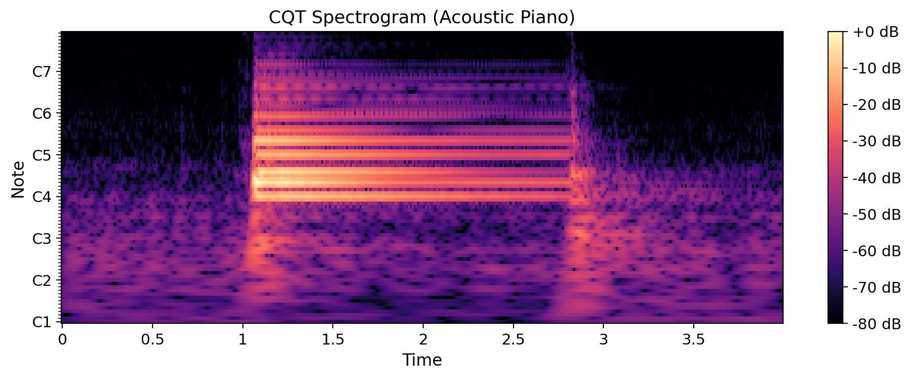
Melody
Melody is a sequence of musical notes perceived as a coherent whole. It is often the most recognisable and memorable part of a piece, and it carries much of how we engage with music emotionally and remember it.
From a psychological perspective, melody is the perception of an organised sequence of tones that form a distinct musical line. The brain tracks pitch contours, intervals, and rhythmic patterns to identify, segment, and remember melodies. This ability underlies our capacity to recognise tunes, anticipate musical phrases, and respond emotionally to music.
Technological advances have enabled detailed analysis and manipulation of melody. Pitch tracking algorithms can extract melodic lines from audio recordings, while MIDI editors and notation software allow for precise editing and visualisation. In music generation and AI composition, models learn melodic patterns from large datasets to create new, stylistically consistent melodies. Melody extraction and similarity algorithms are also used in music search, recommendation systems, and music information retrieval.
Contour and melodic memory
When you recognise a tune, what exactly have you remembered? Research on melodic memory points to a few robust regularities, and most of them can be checked by ear.
- Contour comes first. The up-and-down shape of a melody, its contour, is what listeners retain most reliably from a single hearing. Dowling (1978) showed that listeners accept a new melody as “the same” if it has the same contour and stays in the same scale, even when the exact intervals differ. Only for well-known melodies do the precise intervals matter. This is why a badly sung version of a song is still recognisable. Contour is also what people reproduce when asked to draw a melody in the air: in a RITMO sound-tracing study, participants moved their hands up and down with the pitch in strikingly consistent ways Kelkar & Jensenius, 2018, a link between melody and movement that the body takes further. Singers do it too. In South Indian Karnatak music, vocalists’ hand gestures follow the melodic line so closely that the acceleration of the hand predicts the changes in pitch Pearson & Pouw, 2022, a coupling that Lara Pearson’s SongGesture project at RITMO now compares across vocal traditions.
- High and low are metaphors. In English and Norwegian we call pitches “high” and “low”, and we tend to move a hand upwards with a rising melody. Nothing in a high frequency is physically higher, though. This verticality is a conceptual metaphor, a way of understanding one domain through bodily experience of another Lakoff & Johnson, 1980. Other languages use other images: Farsi speakers describe high pitches as “thin” and low pitches as “thick” Dolscheid et al., 2013.
- Melodies survive transposition. A tune is the same tune in any key, because we hear relative pitch. Memory stores the pattern of intervals and the contour, not the frequencies themselves (except for the few people with absolute pitch, mentioned earlier).
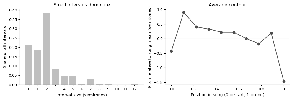
- Small intervals dominate. In melodies from many cultures, most motion is by step, and leaps are rare and mostly small. Huron (2006) attributes this partly to the voice, which finds small intervals easier, and partly to hearing: stepwise motion keeps the notes in one auditory stream (see the section on streams below). Large leaps tend to be followed by a change of direction, a pattern known as gap fill.
- Phrases arch. Phrases tend to rise and then fall, ending lower than they peaked. Together with slowing down and a longer final note, the falling tail of the arch is one of the strongest cues that a phrase is ending.
The figure below checks two of these claims against a real corpus: about 300 German folksongs from the Essen collection, which ships with the music21 toolkit. It counts the size of every melodic interval and plots the average pitch contour across the songs. Because whole songs are averaged rather than single phrases, the arch is flattened in the middle, but the quick rise at the start and the drop to the final note stand out clearly.
Source
import numpy as np
import matplotlib.pyplot as plt
from music21 import corpus
plt.rcParams.update({
    "font.size": 10,
    "axes.titlesize": 11,
    "axes.labelsize": 10,
    "xtick.labelsize": 9,
    "ytick.labelsize": 9,
    "legend.fontsize": 9,
    "figure.figsize": (10, 4),
    "figure.dpi": 100,
    "savefig.dpi": 150,
    "axes.spines.top": False,
    "axes.spines.right": False,
})

songs = corpus.parse("essenFolksong/altdeu10.abc").scores

intervals = []
n_bins = 10
contour_sum, contour_n = np.zeros(n_bins), np.zeros(n_bins)
for song in songs:
    pitches = np.array([n.pitch.midi for n in song.recurse().notes if n.isNote])
    if len(pitches) < 8:
        continue
    intervals += list(np.abs(np.diff(pitches)))              # size in semitones
    relative = pitches - pitches.mean()                       # pitch relative to the song's mean
    position = (np.arange(len(pitches)) / (len(pitches) - 1) * (n_bins - 0.001)).astype(int)
    np.add.at(contour_sum, position, relative)
    np.add.at(contour_n, position, 1)

intervals = np.array(intervals)
steps = np.mean(intervals <= 2)
print(f"{len(songs)} songs, {len(intervals)} melodic intervals; {steps:.0%} are steps of two semitones or less.")

fig, (ax1, ax2) = plt.subplots(1, 2, figsize=(10, 3.5))
sizes = np.arange(0, 13)
ax1.bar(sizes, [np.mean(intervals == s) for s in sizes], color="0.75")
ax1.set_xticks(sizes)
ax1.set_xlabel("Interval size (semitones)")
ax1.set_ylabel("Share of all intervals")
ax1.set_title("Small intervals dominate")

ax2.plot(np.arange(n_bins) / (n_bins - 1), contour_sum / contour_n, marker="o", color="0.3")
ax2.axhline(0, color="0.8", linewidth=0.8)
ax2.set_xlabel("Position in song (0 = start, 1 = end)")
ax2.set_ylabel("Pitch relative to song mean (semitones)")
ax2.set_title("Average contour")
plt.tight_layout()
plt.show()
313 songs, 15189 melodic intervals; 78% are steps of two semitones or less.
Melodic expectation and closure
Just as harmony creates expectation, melody does too. Listeners learn statistical regularities in melodic motion and use them to predict likely continuations.
In tonal contexts, some scale degrees are heard as relatively unstable and often move toward more stable tones. For example, scale degree 7 often resolves to 1, and 2 often moves to 1 near phrase endings. Melodic closure is strengthened by several cues acting together:
- descending or arch-like contour toward phrase end,
- longer final note duration,
- rhythmic deceleration,
- alignment with a cadence in the harmony,
- timbral or dynamic settling.
These cues help explain why some phrases feel complete while others feel open or suspended, even when the pitch material is similar.
The Melody lab app turns these ideas into something you can test. Draw a melody on a pitch grid and play it; the app draws its contour, counts its intervals, and reports how much of it moves by step. It also carries a small statistical model learned from the same Essen folksongs as the figure above: for every note you place, it shows which note the corpus expects next and how surprising your choice was, and a game asks you to guess the next note of a phrase the corpus would write.
Timbre, texture, and musical streams
Pitch and rhythm are only part of what we hear. This last group of topics concerns how simultaneous sounds are held apart or fused together, by timbre, by grouping principles, and by the way parts are layered.
Timbre
Timbre was defined in psychoacoustics as what lets us tell two sounds apart when pitch, loudness, and duration are the same. Here the question is what it does musically.
Timbre strongly influences how we hear both harmony and melody:
- In harmony, timbre affects blending and separation. A chord played by a string quartet can feel fused and smooth, while the same chord split across instruments with contrasting timbres can feel more segmented and tense.
- In melody, timbre helps define identity and continuity. We can often track a melodic line in a dense texture because its timbral profile remains relatively stable over time.
- In polyphonic listening, timbral contrast is one of the key cues for auditory stream segregation, making it easier to separate simultaneous voices.
- In tuning, timbre decides which intervals sound smooth. Two tones are consonant when their partials line up, so a chord that beats audibly on a bright, harmonic-rich synthesiser can sound calm on flutes, and, as the note on non-octave scales showed, a change of timbre can make an entirely different scale sound consonant.
From a technology perspective, timbre is central to music information retrieval and production. Features such as spectral centroid, spectral flux, MFCCs, and temporal envelope descriptors, all numerical summaries of a sound’s spectrum and how it changes over time, are often used to classify instruments, detect playing techniques, and compare recordings. In arrangement and mixing, small timbral changes can alter perceived harmonic clarity, melodic prominence, and emotional impact.
Space
Where sounds come from, and what room they sound in, also shape how harmony and melody are heard.
The auditory system uses direction as a grouping cue, so two lines that come from different places are easier to follow than the same two lines from one loudspeaker. Composers have exploited this for centuries, from antiphonal choirs placed in separate galleries of St Mark’s in Venice to stereo mixes that pan instruments apart so that each line stays audible. The mechanics of spatial hearing were covered in psychoacoustics.
In a reverberant room each chord lingers into the next, so successive chords overlap and are partly heard as one sonority. Music written for cathedrals therefore tends towards slow harmonic rhythm and consonant, sustained textures, while music for dry rooms and close-miked recordings can change harmony quickly and use sharp dissonances without blurring. The room is, in effect, part of the arrangement (see acoustics).
Air absorbs high frequencies, so distant instruments sound darker and fuse more readily with their neighbours. Orchestrators place instruments accordingly, and mixing engineers imitate the effect with filters and reverb to push a part into the background without lowering it much in level.
Streams in musical textures
Albert Bregman’s auditory scene analysis Bregman, 1990 was introduced in psychoacoustics. It explains how the auditory system sorts one incoming pressure wave into separate streams, using cues such as frequency proximity, common onset, continuity, and timbral similarity.
Composers and arrangers work with grouping cues. Lines that stay in separate registers, enter at different moments, or carry contrasting timbres stay audible as independent voices. Lines that share register, attack, and colour fuse into a single chord. That is why one fugue voice remains followable through dense counterpoint, why doubling a melody at the octave thickens it rather than adding a voice, and why an orchestrator can make five instruments sound like one instrument or like five.
The same principles set the ceiling for machines. Automatic transcription and source separation (machine listening) are attempts to solve computationally what the auditory system does effortlessly, and they fail in the places where our own grouping is ambiguous.
The Streaming lab app is the classic experiment behind the figure above, made explorable: two tones alternate, and you set their separation, the tempo, the loudness difference, and the timbre of each, and hear the sequence fall into one stream or two. An experiment mode raises the separation slowly while you press a button at the moment the percept flips, at three tempi, and plots your own boundaries against the reference values from the literature.
Source
import numpy as np
import matplotlib.pyplot as plt
plt.rcParams.update({
    "font.size": 10,
    "axes.titlesize": 11,
    "axes.labelsize": 10,
    "xtick.labelsize": 9,
    "ytick.labelsize": 9,
    "legend.fontsize": 9,
    "figure.figsize": (10, 4),
    "figure.dpi": 100,
    "savefig.dpi": 150,
    "axes.spines.top": False,
    "axes.spines.right": False,
})

# Auditory streaming: the same alternating sequence is heard as one stream or as two,
# depending on how far apart the two tones are in frequency.
ioi, dur, n = 0.12, 0.08, 10
fig, axes = plt.subplots(1, 2, figsize=(10, 3.8), sharey=True)
for ax, (fa, fb, title) in zip(axes, [(400, 450, "Small separation: one stream, a galloping melody"), (400, 1000, "Large separation: two streams, each its own pulse")]):
    times = np.arange(n) * ioi
    freqs = np.where(np.arange(n) % 2 == 0, fa, fb)
    for tt, ff in zip(times, freqs):
        ax.add_patch(plt.Rectangle((tt, np.log2(ff) - 0.06), dur, 0.12, color="C0" if ff == fa else "C1"))
    if fb - fa < 100:
        ax.plot(times + dur / 2, np.log2(freqs), color="0.4", ls="--", lw=1)
    else:
        for ff in (fa, fb):
            sel = freqs == ff; ax.plot(times[sel] + dur / 2, np.log2(freqs[sel]), color="0.4", ls="--", lw=1)
    ax.set_yticks([np.log2(v) for v in (300, 400, 600, 800, 1200)]); ax.set_yticklabels(["300", "400", "600", "800", "1200"])
    ax.set_ylim(np.log2(280), np.log2(1300)); ax.set_xlim(-0.05, n * ioi)
    ax.set_xlabel("Time (s)"); ax.set_title(title, fontsize=10)
axes[0].set_ylabel("Frequency (Hz)")
fig.suptitle("Auditory streaming: the dashed line shows how the tones are heard to connect")
plt.tight_layout()
plt.show()
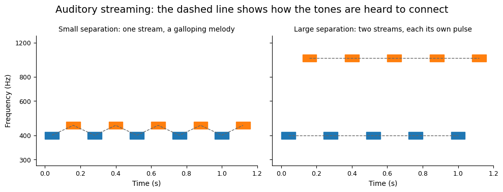
Figure: Auditory streaming. The same alternating sequence of two tones is heard as one galloping melody when the tones are close in frequency (left) and as two separate streams, each with its own slower pulse, when they are far apart (right). The dashed lines show the connections the ear makes. Speeding the sequence up has the same effect as widening the gap.
Gestalt theory in music perception
Auditory grouping draws on Gestalt theory, which explains how humans organise sensory input into meaningful patterns and unified wholes. In music, Gestalt principles help us understand how listeners perceive coherent melodies, phrases, and motifs, even when the acoustic signal is complex or ambiguous.
Key Gestalt principles relevant to music:
- Proximity: Notes close together in time or pitch are grouped as part of the same melodic line.
- Similarity: Notes with similar timbre, loudness, or articulation are perceived as belonging together.
- Continuity: The brain prefers smooth, continuous melodic contours over abrupt changes.
- Closure: Listeners mentally “fill in” missing notes to perceive complete musical phrases.
- Symmetry: Symmetrical patterns or phrases (such as palindromic melodies or balanced phrase structures) are grouped as coherent wholes.
- Figure-Ground: The ability to focus on a primary melody (figure) while treating accompaniment or background sounds as secondary (ground).
These principles interact with auditory stream segregation, allowing us to follow individual voices in polyphonic music, recognise recurring themes, and make sense of complex musical textures. Gestalt theory has influenced both music psychology and computational models for music analysis, providing a framework for understanding how we perceive musical structure and form.
Source
import numpy as np

import matplotlib.pyplot as plt
plt.rcParams.update({
    "font.size": 10,
    "axes.titlesize": 11,
    "axes.labelsize": 10,
    "xtick.labelsize": 9,
    "ytick.labelsize": 9,
    "legend.fontsize": 9,
    "figure.figsize": (10, 4),
    "figure.dpi": 100,
    "savefig.dpi": 150,
    "axes.spines.top": False,
    "axes.spines.right": False,
})

fig, axs = plt.subplots(1, 5, figsize=(10, 2.5))
fig.suptitle("Gestalt Principles in Music Perception")

# Proximity: notes close in pitch/time are grouped
x = np.arange(10)
y = np.concatenate([np.ones(5), np.ones(5)*3])
axs[0].scatter(x, y, s=100, color='dodgerblue')
axs[0].set_title("Proximity")
axs[0].set_xticks([])
axs[0].set_yticks([])

# Similarity: notes with similar color/timbre are grouped
colors = ['dodgerblue']*5 + ['orange']*5
axs[1].scatter(x, np.ones(10)*2, s=100, color=colors)
axs[1].set_title("Similarity")
axs[1].set_xticks([])
axs[1].set_yticks([])

# Continuity: smooth melodic contour
x = np.linspace(0, 9, 100)
y = np.sin(x/2) + 2
axs[2].plot(x, y, color='dodgerblue', lw=3)
axs[2].set_title("Continuity")
axs[2].set_xticks([])
axs[2].set_yticks([])

# Closure: incomplete phrase, brain fills gap
axs[3].plot([0, 1, 2, 3], [2, 3, 2, 1], 'o-', color='dodgerblue', lw=2)
axs[3].plot([3, 4], [1, 2], 'o--', color='dodgerblue', lw=2, alpha=0.5)
axs[3].set_title("Closure")
axs[3].set_xticks([])
axs[3].set_yticks([])

# Symmetry: palindromic phrase
y = [1, 2, 3, 2, 1]
axs[4].plot(range(5), y, 'o-', color='dodgerblue', lw=2)
axs[4].set_title("Symmetry")
axs[4].set_xticks([])
axs[4].set_yticks([])

plt.tight_layout(rect=[0, 0, 1, 0.93])
plt.show()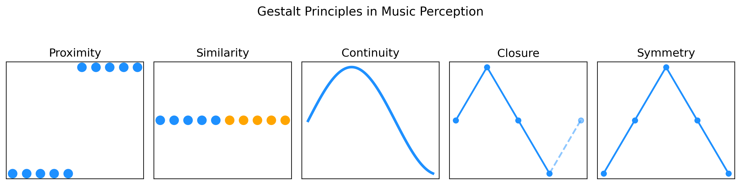
Musical auditory illusions
Psychoacoustics covered illusions that arise from the mechanics of hearing: masking, the missing fundamental, and the endless Shepard tone. The illusions here are musical, since they need scales, intervals, and two-handed textures to work at all.
Diana Deutsch is a psychologist whose experiments on auditory illusions Deutsch, 1991 have uncovered perceptual phenomena that reveal how our brains organise and interpret complex sound patterns. Some of her most famous auditory illusions include:
The Tritone Paradox: When two tones separated by a tritone (half an octave) are played in succession, some listeners perceive the sequence as ascending in pitch, while others hear it as descending. The direction of the perceived pitch change can vary depending on the listener’s linguistic background and even their geographical origin, suggesting that pitch perception is influenced by both biology and experience.
The Octave Illusion: When two tones an octave apart are alternately played to each ear (for example, high tone to the right ear, low tone to the left, then switching), listeners often perceive a single tone that alternates between ears and changes pitch, even though both tones are always present. This illusion demonstrates how the brain integrates and separates auditory information from both ears.
The Scale Illusion: When ascending and descending musical scales are split between the two ears (with some notes sent to the left ear and others to the right), listeners tend to perceive coherent melodic lines that do not correspond to the actual physical input. The brain “reconstructs” the most plausible musical pattern, illustrating its tendency to organise sounds into familiar structures.
Phantom Tones: In this illusion, repeating ambiguous speech sounds can cause listeners to “hear” words or phrases that are not actually present. The specific words perceived can vary between individuals, highlighting the role of expectation, language, and context in auditory perception.
Deutsch’s work demonstrates that auditory perception is not a simple reflection of the physical properties of sound, but an active process shaped by cognitive, cultural, and neural factors. Her illusions are widely used in research, education, and demonstrations to illustrate how we hear and interpret sound.
For more examples and audio demonstrations, visit Diana Deutsch’s Auditory Illusions website. In the lecture below, Musical Illusions and Phantom Words, recorded by the Acoustical Society of America, Deutsch demonstrates some of these illusions herself:
Texture
The last concept in this group is texture, a term used to describe the overall complexity and character of a “musical soundscape.” Texture refers to how musical lines, timbres, and harmonies are layered and interact within a piece of music.
Vertical dimension: Texture describes the layering of different timbres and pitches at a given moment. For example, the combined sound of multiple instruments in an orchestra, or the blend of voices in a choir, creates a rich and complex vertical texture. The number of simultaneous parts, their timbral qualities, and their harmonic relationships all contribute to the perceived thickness or thinness of the texture.
Horizontal dimension: Texture also refers to how melodic lines combine and interact over time. In monophonic textures, there is a single melodic line with no accompaniment. Homophonic textures feature a primary melody supported by chords or harmonies. Polyphonic textures involve two or more independent melodic lines occurring simultaneously, as in a fugue or canon. Heterophonic textures occur when multiple performers play variations of the same melody at the same time.
Texture can change throughout a piece, creating contrast and interest. Composers use texture to shape musical form, highlight important moments, and evoke different emotional responses. In modern music production, texture is also shaped by mixing techniques, effects, and the spatial placement of sounds.
A critical look: is consonance preference universal?
Textbooks often treat the preference for consonance over dissonance as a human universal, grounded in the harmonic series. That claim is testable, but only with listeners who have not grown up surrounded by Western harmony.
- The claim is that people everywhere prefer consonant combinations, such as octaves and fifths, to dissonant ones, such as seconds and tritones.
- The evidence comes from a field study with the Tsimane’, an Amazonian society with little exposure to Western music McDermott et al., 2016. Tsimane’ listeners rated consonant and dissonant chords as equally pleasant, while listeners in the United States, and Bolivian town and city dwellers with intermediate exposure, preferred consonance roughly in proportion to that exposure.
- The method used headphone-based pleasantness ratings of sung and synthesised intervals, with control tasks confirming that the Tsimane’ heard the difference perfectly well and disliked acoustic roughness. They discriminated; they simply did not prefer.
- The limits are one population, unfamiliar rating tasks, and an ongoing debate, since later studies have argued for partial preferences or questioned aspects of the design. One striking study cannot settle a nature-versus-nurture question on its own.
What survives is important enough: the aesthetic value attached to consonance appears to be learned, at least in part, from the music around you. The consonance ranking game in the Interval lab lets you compare your own ratings with typical Western ones.
- Shepard, R. N. (1964). Circularity in Judgments of Relative Pitch. The Journal of the Acoustical Society of America, 36(12), 2346–2353. 10.1121/1.1919362
- Krumhansl, C. L. (2001). Cognitive Foundations of Musical Pitch. Oxford University Press. 10.1093/acprof:oso/9780195148367.001.0001
- Pearson, L. (2013). Gesture and the Sonic Event in Karnatak Music. Empirical Musicology Review, 8(1), 2–14. 10.18061/emr.v8i1.3918
- Mathews, M. V., Pierce, J. R., Reeves, A., & Roberts, L. A. (1988). Theoretical and Experimental Explorations of the Bohlen–Pierce Scale. The Journal of the Acoustical Society of America, 84(4), 1214–1222. 10.1121/1.396622
- Sethares, W. A. (2005). Tuning, Timbre, Spectrum, Scale (2nd ed.). Springer. 10.1007/b138848
- Huron, D. (2006). Sweet Anticipation: Music and the Psychology of Expectation. The MIT Press. 10.7551/mitpress/6575.001.0001
- Margulis, E. H. (2018). The Psychology of Music: A Very Short Introduction. Oxford University Press. 10.1093/actrade/9780190640156.001.0001
- Dowling, W. J. (1978). Scale and Contour: Two Components of a Theory of Memory for Melodies. Psychological Review, 85(4), 341–354. 10.1037/0033-295X.85.4.341
- Kelkar, T., & Jensenius, A. (2018). Analyzing Free-Hand Sound-Tracings of Melodic Phrases. Applied Sciences, 8(1), 135. 10.3390/app8010135
- Pearson, L., & Pouw, W. (2022). Gesture–vocal coupling in Karnatak music performance: A neuro–bodily distributed aesthetic entanglement. Annals of the New York Academy of Sciences, 1515(1), 219–236. 10.1111/nyas.14806
- Lakoff, G., & Johnson, M. (1980). Metaphors We Live By. University of Chicago Press.
- Dolscheid, S., Shayan, S., Majid, A., & Casasanto, D. (2013). The Thickness of Musical Pitch: Psychophysical Evidence for Linguistic Relativity. Psychological Science, 24(5), 613–621. 10.1177/0956797612457374
- Bregman, A. S. (1990). Auditory Scene Analysis: The Perceptual Organization of Sound. The MIT Press. 10.7551/mitpress/1486.001.0001
- Deutsch, D. (1991). The Tritone Paradox: An Influence of Language on Music Perception. Music Perception, 8(4), 335–347. 10.2307/40285517
- McDermott, J. H., Schultz, A. F., Undurraga, E. A., & Godoy, R. A. (2016). Indifference to Dissonance in Native Amazonians Reveals Cultural Variation in Music Perception. Nature, 535(7613), 547–550. 10.1038/nature18635