Music unfolds in time. Rhythm and metre depend on duration, order, and recurrence. They give us the structures we use to predict, move, and coordinate. This chapter begins with broad ideas of time and rhythm, then turns to timing, the question of when a single sound happens. From there it turns to pulse and tempo, to entrainment as the mechanism that lets us move to a beat, and to metre as the hierarchy that entrainment builds. We then zoom in on microrhythmic nuance and end with the phenomenon of groove. This chapter runs across all the four levels of description. An onset is a physical event you can find in a waveform; a perceptual centre is where the ear puts it; a backbeat that feels laid-back rather than late is interpretation. Here, we will explore how they compare.
Time
Time in music refers to the organisation of sounds and silences in a temporal framework. It is the foundation on which rhythm, beat, and metre are built. Musical time is also more than clock measurement: it is shaped by perception, culture, and performance practice. Rhythms and metres may be notated in a score, but their feel depends on how musicians and listeners interpret and embody them.
Time scales
Sound and music span a range of time scales, and different scales are handled by different parts of the hearing system and the brain. The figure below lays them out on a logarithmic axis, where each step is ten times longer than the last. At the fast end sit differences of a few tens of microseconds between the two ears, which the auditory system uses to locate a sound source (see psychoacoustics). Waveform periods between about 0.05 and 50 ms are heard as pitch rather than as separate events. After that, we start hearing individual events, and rhythmic structures may emerge.
Source
import numpy as np
import matplotlib.pyplot as plt
plt.rcParams.update({
    "font.size": 10,
    "axes.titlesize": 11,
    "axes.labelsize": 10,
    "xtick.labelsize": 9,
    "ytick.labelsize": 9,
    "legend.fontsize": 9,
    "figure.figsize": (10, 4),
    "figure.dpi": 100,
    "savefig.dpi": 150,
    "axes.spines.top": False,
    "axes.spines.right": False,
})

# Approximate ranges, in seconds, for illustration only.
music = [
    ("Interaural time difference", 1e-5, 7e-4),
    ("Perceived pitch", 5e-5, 5e-2),
    ("Microrhythm", 5e-3, 1e-1),
    ("Subdivisions", 1e-1, 5e-1),
    ("Beat", 3e-1, 1.5),
    ("Bar and phrase", 1.5, 10),
    ("Sections and whole pieces", 30, 3600),
]
body = [
    ("Running", 0.3, 0.4),
    ("Walking", 0.4, 0.7),
    ("Heartbeat at rest", 0.6, 1.2),
    ("Respiration", 3, 6),
    ("Periodic machines (e.g. fridges)", 300, 3600),
    ("Sleep\u2013wake cycle", 7e4, 1.05e5),
    ("Menstrual and lunar cycles", 2.0e6, 3.0e6),
    ("Annual cycle", 2.9e7, 3.4e7),
]
rows = [(n, lo, hi, "steelblue") for n, lo, hi in music] + \
       [(n, lo, hi, "darkorange") for n, lo, hi in body]

fig, ax = plt.subplots(figsize=(10, 5))
ax.axvspan(0.2, 1.8, color="0.92", zorder=0)
ax.text(np.sqrt(0.2 * 1.8), len(rows) - 0.4, "perceived rhythm\n(Fraisse, 200\u20131800 ms)",
        ha="center", va="bottom", color="0.4", fontsize=9)
for i, (name, lo, hi, col) in enumerate(rows):
    y = len(rows) - 1 - i
    ax.barh(y, hi - lo, left=lo, height=0.55, color=col, alpha=0.85, zorder=3)
    ax.text(lo / 1.6, y, name, ha="right", va="center")
ax.set_xscale("log")
ticks = [1e-5, 1e-4, 1e-3, 1e-2, 1e-1, 1, 10, 60, 600, 3600, 86400, 2.6e6, 3.15e7]
labels = ["10 \u00b5s", "100 \u00b5s", "1 ms", "10 ms", "100 ms", "1 s", "10 s",
          "1 min", "10 min", "1 h", "1 day", "1 month", "1 year"]
ax.set_xticks(ticks)
ax.set_xticklabels(labels)
ax.set_xlim(2e-8, 1e8)
ax.set_ylim(-0.7, len(rows) + 1.0)
ax.set_yticks([])
ax.spines["left"].set_visible(False)
ax.set_xlabel("Duration or period (logarithmic axis)")
ax.set_title("Time scales in sound, music (blue), the body, and the surroundings (orange)")
plt.tight_layout()
plt.show()
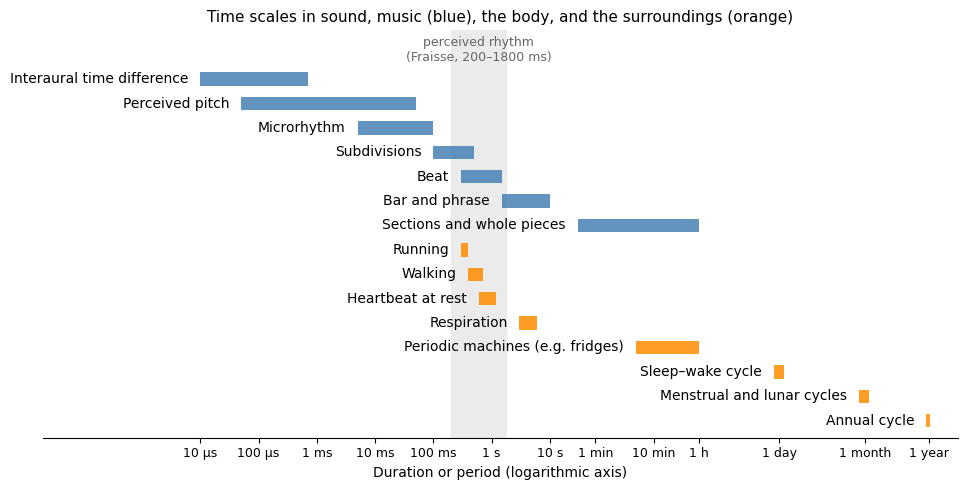
Figure: Time scales of sound and music (blue) and of the body and its surroundings (orange) on a logarithmic axis. The grey band marks the range in which Fraisse placed perceived rhythm. The ranges are approximate and drawn for orientation, not measured.
The psychologist Paul Fraisse distinguished between rhythms that are perceived and rhythms that are conceived Fraisse, 1982. Perceived rhythms have intervals of roughly 200–1800 ms, which is the range of subdivisions, beats, and short groupings. Faster events fuse into a single sound: you can hear this happen with the From pulse to pitch app, where a click repeated faster and faster turns from a series of pulses into a buzzing tone once the gaps are shorter than a few tens of milliseconds. Slower cycles have to be counted or remembered rather than felt. The upper limit is related to the few seconds that auditory short-term memory can hold at once, which is also about the length of a musical phrase.
Dig deeper: the layers of memory
Bob Snyder separates memory into layers that line up with the scales in the figure Snyder, 2000:
- Echoic memory holds the raw sound for a fraction of a second. It is what fuses fast events into a single tone with a pitch, and it is where the ear decides when an attack begins.
- Short-term memory holds about 3–5 s, a little more with rehearsal, and only about seven items at a time, the “magical number seven, plus or minus two” Miller, 1956. This is the span of a phrase and of a metric cycle, and the reason a rhythm has to repeat within a few seconds to be felt rather than counted.
- Working memory is the active part of short-term memory: counting beats, holding the pattern of one bar while playing the next, comparing a repetition with the one before.
- Long-term memory holds minutes to years: the form of a piece, the metres and grooves of a style learned over a lifetime, and the expectations a listener brings before the first note. Slower cycles are conceived here rather than perceived.
Snyder ties these layers to three levels of musical experience: event fusion, melodic and rhythmic grouping, and form. Most of this chapter lives in the middle level.
The body keeps time at several of these scales too. Walking steps come about twice a second and running steps about three times a second, the heart beats about once a second at rest, and a breath takes around four seconds. Slower still are the cycles that chronobiology studies Koukkari & Sothern, 2006: hormonal rhythms of an hour or two, the 24-hour sleep–wake cycle, the menstrual cycle of about a month, close to the lunar cycle, and the annual cycle of the seasons that governs migration and hibernation. None of these are perceived as rhythms in Fraisse’s sense, but they form the background against which musical time is experienced, and they can couple to music, as the sections on entrainment below and the chapter on physiology show. At the slow end of the axis, the appliances in a room switch on and off with periods of minutes, a case we return to at the end of the chapter.
Clock time and felt time
A clock measures duration; a listener feels it. Psychologists separate judgements of duration, how long something lasted, from judgements of the passage of time, whether it seemed to pass quickly or slowly Wearden, 2015. The two do not always agree. A three-minute song and three minutes of silence have the same duration, but they are not felt to be the same length, and a long concert can pass in a flash while a short wait feels endless. The classic explanation is an internal clock whose ticks are counted and compared with memory, so that a faster clock, driven by arousal or attention, makes an interval feel longer Allman et al., 2014. More recent accounts suggest that the brain keeps several parallel timelines that are recalibrated as events unfold rather than one central clock.
Rhythm
What is rhythm? Everyone knows one when they hear it, yet the word is hard to pin down. At its most general, rhythm is about repetition. In biology it has been defined as “a change that is repeated with a similar pattern” Koukkari & Sothern, 2006, and Anne Danielsen, borrowing a phrase from the poet Amiri Baraka, describes musical rhythm as a “changing same” Danielsen, 2010. Both definitions include the heartbeat, the tides, and a fridge switching on and off, and this chapter uses rhythm in that broad sense whenever it looks beyond music.
In music the term usually means something narrower: a pattern of durations formed by the intervals between the perceived time points of notes. Notice the word perceived. A rhythm is not the sound signal itself but the pattern of time points a listener hears in it. This is why the same recording can be heard as several rhythms, and why the perceptual centre of a sound, discussed later in this chapter, matters as much as its physical onset.
Rhythm in notation
Western notation writes such patterns of durations with note values. Each value is half the length of the one before it, from the whole note down through half, quarter, eighth, and sixteenth notes, and every value has a rest of the same length for silence. A dot extends a value by half, and a tuplet squeezes three notes into the time of two. Note values say nothing about how long a note lasts in seconds; that is fixed only when a tempo is chosen.
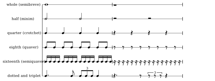
Figure: Note values and rests in Western notation. Each row fills one bar of 4/4 with twice as many notes as the row above, so the halving lines up vertically, and the second bar of each row shows the rest of the same length. The last row shows a dotted quarter and a triplet.
Rhythms can be periodic (based on cycles, such as a metronome) or aperiodic (irregular, as in speech or improvisation). Both can be meaningful: a drum groove in 4/4 and a free jazz solo each have rhythm, but in different senses.
Rhythms also carry cultural meaning. A clave rhythm in Afro-Cuban music is more than a sequence of durations; it is a structural reference for musicians and dancers. In the same way, speech rhythms shape the flow of rap and spoken-word performance.
Rhythm as a signal
Rhythms are often drawn as points on a timeline, but both bodily and musical rhythms are carried by continuous signals that can vary in the three ways we discussed in the acoustics chapter: period (time taken by one cycle), amplitude (strength of each cycle), and its phase (the position within the cycle at a given moment). All three return later in the chapter: the period sets the tempo, differences in amplitude mark the accents of a metre, and phase is what a tapping finger aligns when it entrains to a beat.
“Perfect” rhythms are rare. A metronome comes close, but few people would call a metronome musical. What makes music interesting is that its rhythms are not perfect. Much of the research presented in this chapter, from tapping to swing, is about how much, and in what way, real rhythms depart from perfect ones.
Rhythm is also tied to movement. Eric Clarke argues that rhythm and timing can be “seen as the consequence of movement, and rhythm and timing seen as the source of, or motivation for, movement” Clarke, 1999. That two-way link between hearing a rhythm and moving to it runs through the sections on tempo, entrainment, and groove.
Timing
In rhythm studies, it is crucial to say when a sound happens. This is a much harder question than it sounds. A sound has a physical onset that can be found in the waveform, a moment at which the ear places it, and several landmarks in between. The distance between these is small, often a few tens of milliseconds, but it is the same size as the timing differences that give music its feel, so it has to be sorted out first.
Onset timing
When we speak of the “timing” of instruments in performance, we usually mean onset timing: when each sound begins. In a recording, the physical onset is the moment the waveform starts to rise out of the silence or the background. Finding it automatically is a standard task in audio analysis, and the algorithms for it are treated in machine listening. A sound has other timing landmarks too:
- Physical onset: the moment the sound begins in the waveform
- Energy peak: the moment the sound is loudest
- Attack time: the time from the physical onset to the energy peak
- Perceptual centre: the moment the ear places the sound at, which is the subject of the next section
Source
import numpy as np
import matplotlib.pyplot as plt
plt.rcParams.update({
    "font.size": 10,
    "axes.titlesize": 11,
    "axes.labelsize": 10,
    "xtick.labelsize": 9,
    "ytick.labelsize": 9,
    "legend.fontsize": 9,
    "figure.figsize": (10, 4),
    "figure.dpi": 100,
    "savefig.dpi": 150,
    "axes.spines.top": False,
    "axes.spines.right": False,
})

t = np.linspace(0, 1.0, 2000)
onset = 0.10
rise = np.clip((t - onset) / 0.10, 0, 1)
attack = rise ** 2 * (3 - 2 * rise)                          # smooth rise from onset to peak
decay = np.exp(-(t - 0.20) / 0.22) * (t >= 0.20) + (t < 0.20)
shoulder = 0.25 * np.exp(-((t - 0.45) / 0.08) ** 2)         # a second bump, as in a real tone
env = attack * decay + shoulder * (t > 0.2)
env /= env.max()

t_peak = t[np.argmax(env)]
t_centroid = np.sum(t * env) / np.sum(env)
t_perc_onset = onset + 0.02
t_perc_attack = onset + 0.065

fig, ax = plt.subplots(figsize=(10, 4))
ax.fill_between(t, env, color="steelblue", alpha=0.15)
ax.plot(t, env, color="steelblue", linewidth=2)
marks = [
    (onset, "Physical onset\n(signal rises above threshold)", 0.05, 0.25),
    (t_perc_onset, "Perceptual onset\n(earliest moment heard)", 0.05, 0.55),
    (t_perc_attack, "Perceptual attack / P-centre\n(where the ear places the event)", 0.05, 0.88),
    (t_peak, "Energy peak", 0.55, 1.08),
    (t_centroid, "Temporal centroid\n(balancing point of the energy)", 0.55, 0.72),
]
for x, label, tx, ty in marks:
    ax.axvline(x, color="0.4", linestyle=":", linewidth=1)
    ax.annotate(label, xy=(x, min(ty, 1.0)), xytext=(tx, ty),
                ha="right" if tx < x else "left", va="center", color="0.25",
                arrowprops=dict(arrowstyle="-", color="0.6", linewidth=0.8))
ax.annotate("", xy=(onset, -0.08), xytext=(t_peak, -0.08),
            arrowprops=dict(arrowstyle="<->", color="0.3"))
ax.text((onset + t_peak) / 2, -0.13, "attack time", ha="center", color="0.3")
ax.set_xlim(-0.3, 1.0)
ax.set_xticks(np.arange(0, 1.01, 0.2))
ax.set_ylim(-0.18, 1.2)
ax.set_yticks([])
ax.spines["left"].set_visible(False)
ax.set_xlabel("Time (s)")
ax.set_title("Timing landmarks of a single sound event: the event has no single \"moment\"")
plt.tight_layout()
plt.show()
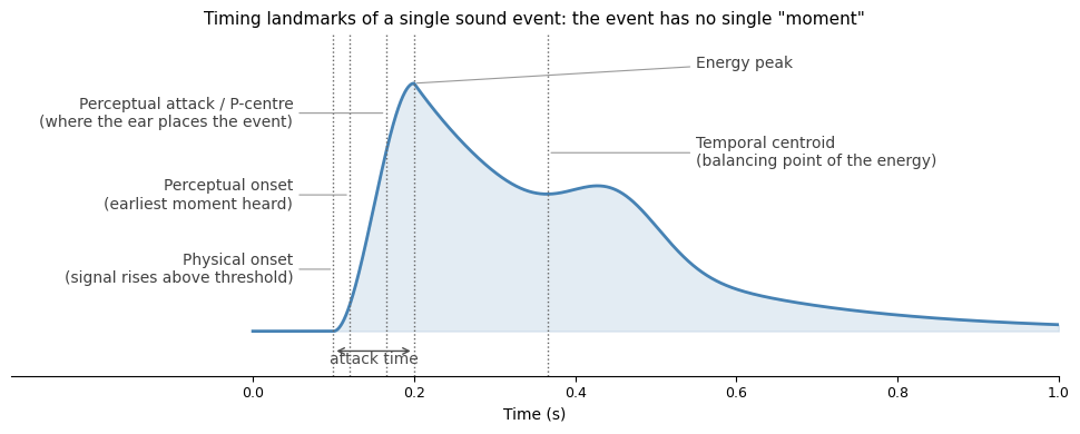
Figure: The amplitude envelope of one tone with the timing landmarks used in rhythm research. Schematic, after Nymoen et al. (2017).
Perceptual centre and attack time
When listening to rhythms, the “moment of occurrence” of a sound, the point we use to place it in time, often does not coincide with its physical onset. This percept is usually called the perceptual centre (P-centre) or perceived attack time (PAT): a subjective reference point that typically falls somewhere after the physical onset and before the peak of the sound’s energy.
Studies show that certain sound parameters affect where P-centres are heard. Attack duration or time (from onset to peak) is the strongest factor: faster attacks yield earlier P-centres, and slower attacks yield later ones. Total duration (from onset to offset) has a weaker but similar influence, with shorter sounds shifting P-centres earlier and longer sounds shifting them later. A RITMO study that varied the attack, duration, and frequency of drum sounds and synthetic tones confirmed this pattern, and also found that slow-attack sounds have a wider, less precise P-centre Danielsen et al., 2019. Anne Danielsen describes the consequence as a beat bin: the beat is not a point in time but a window, and the sounds that mark it decide how wide the window is.
Source
import numpy as np
import matplotlib.pyplot as plt
plt.rcParams.update({
    "font.size": 10,
    "axes.titlesize": 11,
    "axes.labelsize": 10,
    "xtick.labelsize": 9,
    "ytick.labelsize": 9,
    "legend.fontsize": 9,
    "figure.figsize": (10, 4),
    "figure.dpi": 100,
    "savefig.dpi": 150,
    "axes.spines.top": False,
    "axes.spines.right": False,
})

t = np.linspace(0, 0.6, 1200)

def envelope(attack, duration):
    rise = np.clip(t / attack, 0, 1) ** 2
    fall = np.clip((duration - t) / (0.25 * duration), 0, 1)
    return rise * fall

cases = [
    ("Fast attack, short duration", 0.01, 0.20, 0.018),
    ("Slow attack, long duration", 0.12, 0.55, 0.095),
]
fig, axes = plt.subplots(1, 2, figsize=(10, 3.2), sharey=True)
for ax, (name, attack, duration, pcentre) in zip(axes, cases):
    env = envelope(attack, duration)
    ax.fill_between(t, env, color="steelblue", alpha=0.25)
    ax.plot(t, env, color="steelblue", linewidth=2)
    ax.axvline(0, color="0.4", linestyle=":", linewidth=1)
    ax.axvline(pcentre, color="darkorange", linestyle="--", linewidth=2)
    ax.text(-0.012, 1.12, "physical onset", color="0.4")
    ax.text(pcentre + 0.012, 0.4, f"P-centre\n{pcentre * 1000:.0f} ms after onset", color="darkorange")
    ax.set_title(name)
    ax.set_xlim(-0.02, 0.6)
    ax.set_ylim(0, 1.25)
    ax.set_yticks([])
    ax.spines["left"].set_visible(False)
    ax.set_xlabel("Time (s)")
axes[0].text(0.35, 0.5, "earlier P-centre", color="0.3", ha="center")
axes[1].text(0.45, 0.6, "later P-centre", color="0.3", ha="center")
plt.suptitle("Faster attacks and shorter sounds are heard earlier relative to their physical onset")
plt.tight_layout()
plt.show()
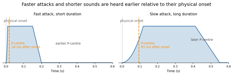
Figure: Two sounds starting at the same instant. The ear places the sharp, short one almost at its onset and the slow, long one well after it. Schematic; the millisecond values are illustrative.
Timbre and timing
The P-centre results have a practical consequence: what plays affects when it is heard. Here, the timbre of the instruments (its sound “colour”) is important. Because the P-centre depends on the attack, two musicians who want to sound together cannot simply start their notes at the same instant. A bassist with a soft, round attack has to play slightly ahead of a drummer’s sharp snare stroke for the two to be heard as synchronous, and a choir, whose consonants take time to form, will sound behind a piano unless the singers anticipate. Producers meet the same problem from the other side: lining up tracks by their waveform onsets in a digital audio workstation does not guarantee that they sound “tight”, so many align by ear instead. Timbre also decides how precisely timing can be judged at all.
Take two guitar chords, one played by slowly arpeggiating the strings (“swept”) and one played by stroking all the strings in quick succession (“swift”). Although both come from the same instrument, the swept stroke tends to sound as if it occurs slightly later relative to its physical onset, while the swift stroke has a P-centre much closer to its onset timing.
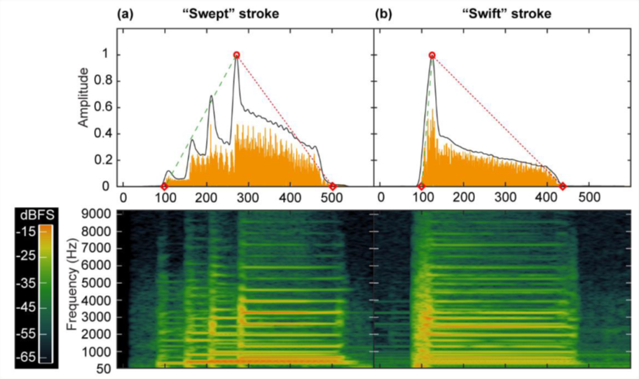
Image source: adapted from Câmara et al. (2020).
The figure below shows the consequence for a sequence. Three identical sounds with evenly spaced onsets sound evenly spaced (A). Replace the middle one with a slow-attack sound and the onsets are still even, but its P-centre falls late, so the sequence sounds uneven (B). The same holds for sounds that start together: they sound together only if their P-centres coincide, not their onsets.
Source
import numpy as np
import matplotlib.pyplot as plt
plt.rcParams.update({
    "font.size": 10,
    "axes.titlesize": 11,
    "axes.labelsize": 10,
    "xtick.labelsize": 9,
    "ytick.labelsize": 9,
    "legend.fontsize": 9,
    "figure.figsize": (10, 4),
    "figure.dpi": 100,
    "savefig.dpi": 150,
    "axes.spines.top": False,
    "axes.spines.right": False,
})

t = np.linspace(0, 3.2, 3200)

def envelope(start, attack, duration):
    x = t - start
    rise = np.clip(x / attack, 0, 1) ** 2
    fall = np.clip((duration - x) / (0.2 * duration), 0, 1)
    return rise * fall * (x >= 0)

onsets = [0.2, 1.2, 2.2]                                         # equal IOIs of 1.0 s
rows = [
    ("A. Physically isochronous and perceptually isochronous",
     [(0.01, 0.5, 0.02)] * 3),
    ("B. Physically isochronous but perceptually non-isochronous",
     [(0.01, 0.5, 0.02), (0.45, 0.6, 0.38), (0.01, 0.5, 0.02)]),
]
fig, axes = plt.subplots(2, 1, figsize=(10, 5.2), sharex=True)
for ax, (title, sounds) in zip(axes, rows):
    pcentres = []
    for start, (attack, duration, offset) in zip(onsets, sounds):
        env = envelope(start, attack, duration)
        ax.fill_between(t, env, color="steelblue", alpha=0.25)
        ax.plot(t, env, color="steelblue", linewidth=1.5)
        ax.axvline(start + offset, color="darkorange", linestyle="--", linewidth=1.8)
        pcentres.append(start + offset)
    for k in range(2):                                            # IOI brackets above
        ax.annotate("", xy=(onsets[k], 1.25), xytext=(onsets[k + 1], 1.25),
                    arrowprops=dict(arrowstyle="|-|", color="0.35", mutation_scale=3))
        ax.text((onsets[k] + onsets[k + 1]) / 2, 1.32,
                f"IOI = {onsets[k + 1] - onsets[k]:.2f} s", ha="center", color="0.35")
        ax.annotate("", xy=(pcentres[k], -0.25), xytext=(pcentres[k + 1], -0.25),
                    arrowprops=dict(arrowstyle="|-|", color="darkorange", mutation_scale=3))
        ax.text((pcentres[k] + pcentres[k + 1]) / 2, -0.45,
                f"IPI = {pcentres[k + 1] - pcentres[k]:.2f} s", ha="center", color="darkorange")
    ax.set_title(title, loc="left")
    ax.set_ylim(-0.6, 1.5)
    ax.set_yticks([])
    ax.spines["left"].set_visible(False)
axes[1].set_xlabel("Time (s)")
plt.tight_layout()
plt.show()
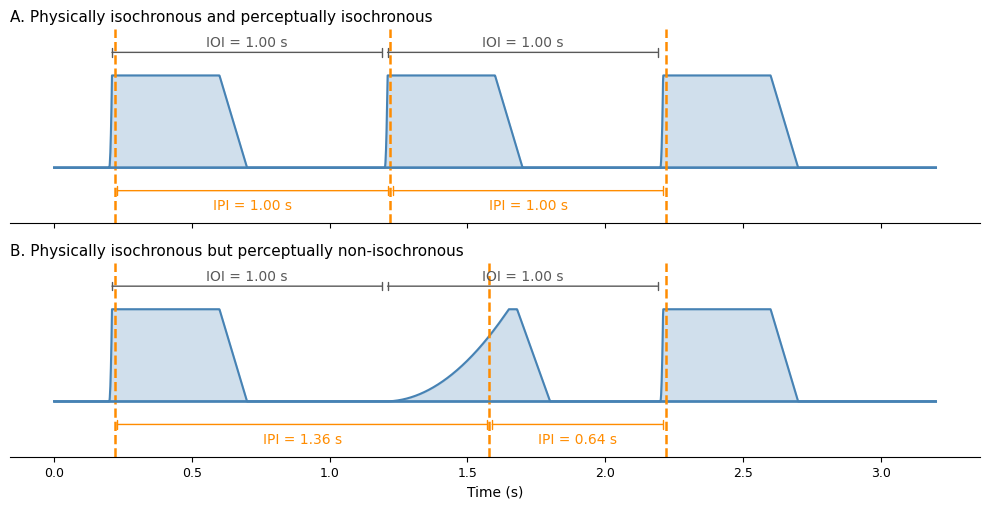
Figure: Three sounds with identical onset spacing. In A they also sound evenly spaced. In B the middle sound has a slow attack, its P-centre (dashed) falls late, and the sequence sounds uneven even though the onsets are not. Schematic, after Villing (2010).
Space and timing
Recall from acoustics that sound travels at about 343 metres per second. Two musicians 10 metres apart therefore hear each other about 30 ms late, which is more than the asynchronies that give a groove its feel. In a symphony orchestra the distance from the double basses to the first violins can exceed 20 metres, which is one reason players follow the conductor’s visible beat rather than the sound from the far side of the stage.
The same problem appears when musicians play together over a network. In experiments where two people clapped a rhythm together through an artificial delay, tempo stayed stable up to a delay of roughly 10 to 20 ms and then slowed steadily as the delay grew, because each player waited for the other Chafe et al., 2010.
Rooms add an additional spatial effect. Reverberation prolongs every sound and smears the onsets that timing perception depends on, so fast, detailed rhythms that are crisp in a dry studio become a wash in a cathedral. Music written for reverberant spaces tends, accordingly, to move slowly.
Pulse and tempo
With the timing of single sounds settled, we can turn to the regular series of them that a listener feels as a beat, to how fast it goes, and to the rate at which the body would set it on its own.
Pulse
The beat (also called the tactus or pulse) is the basic time unit of music: the regular series of moments that a listener feels the music moving in. A pulse can also describe an ongoing stream of beats; one can speak of 8th-note pulses just as much as quarter-note pulses. Either way, the beat level is what we naturally tap our feet to, giving stability and predictability to performers and listeners alike.
Research suggests that we comfortably perceive and move to beats when the time between them (the inter-onset interval, IOI) lies between about 500 and 700 ms, that is, 86–120 BPM. Pulse is thus closely tied to our sensorimotor system: we tend to move along with it. Faster events are heard as subdivisions, and slower ones are grouped into larger spans.
Note that in music, the pulse is not always marked by sound. Even when silent, it can be inferred as a virtual reference that organises events. Musicians often “feel” the pulse even when they play around it.
You can explore this with the Silent beats app, which loops one bar of 4/4 with a pulse of four clicks and a rhythm on a grid of sixteenths. Any click or event can be silenced, the pulse can drop out for whole bars, and the rhythm can be rotated against the beat, so that the same durations fall on different levels of the metric hierarchy.
Tempo
Tempo is the rate of the beat, measured in beats per minute (BPM). In notation the beat is often the quarter note, but the tempo is a property of what is heard, not of how it is written.
Scores give the tempo either as a metronome marking such as ♩ = 120, exact in beats per minute, or as an Italian tempo marking such as andante, which names a character as much as a speed.
Dig deeper: tempo markings
Western scores have marked tempo in two ways. Since the early 1800s a metronome marking such as ♩ = 120 has given the beat rate exactly, in beats per minute, a practice that spread with Maelzel’s clockwork metronome and that Beethoven took up at once. Older, and still more common, are the Italian tempo markings, which name a character as much as a speed. The table gives the conventional ranges printed on metronomes; they vary between sources and periods, and a marking such as andante, from the Italian for walking, says how the music should move rather than exactly how fast.
| Marking | Meaning | Conventional range (BPM) |
|---|---|---|
| Largo | broad | 40–60 |
| Adagio | at ease | 66–76 |
| Andante | walking | 76–108 |
| Moderato | moderate | 108–120 |
| Allegro | lively | 120–156 |
| Vivace | brisk | 156–176 |
| Presto | very fast | 168–200 |
Markings also change tempo within a piece: accelerando and ritardando for a gradual speeding up or slowing down, and rubato, literally stolen time, for the performer’s freedom to stretch and compress the beat expressively. All of these describe the beat level; the subdivisions and bars scale with it.
Spontaneous motor tempo
Recall the exercise at the beginning of this chapter. When done in controlled studies, most people will settle at around 100–120 BPM, an interval of roughly 500–600 ms between taps. This rate is called the spontaneous motor tempo (SMT) Fraisse, 1982. It varies between people, is fairly stable within a person from day to day, and slows with age.
The spontaneous motor tempo also matches the rate of walking, and sits close to the tempo at which people most easily hear and follow a beat, which peaks at around 120 BPM Moelants, 2002. Much dance music lives in the same range, or a little faster, to “make” you move.
The overlap between tapping, walking, and preferred musical tempo is one of the clearest signs that musical time is rooted in the moving body. Tapping is also the standard laboratory task for studying timing: in sensorimotor synchronisation experiments, people tap along with a metronome and the timing of each tap is measured against the click Repp, 2005. How the body produces timing, from tapping to whole-body movement, is the subject of a section in the body.
Entrainment
Entrainment refers to the synchronisation of a person’s movements or internal rhythms with an external rhythm, such as a musical beat. This is the course’s main treatment of the idea, so it is worth stating in its general form before we narrow it to music.
Coupled oscillators
The underlying physics is that of coupled oscillators: two systems that influence each other, however weakly, tend to fall into a stable phase or frequency relationship rather than drift independently. The first recorded case had nothing to do with music: in 1665 Christiaan Huygens noticed that two pendulum clocks hanging from the same beam fell into step with each other, and found that the tiny vibrations travelling through the beam were enough to hold them there. Nothing about that is specific to music, or even to biology. What makes it useful here is that a great many things about a person oscillate, including attention, limb movement, breathing, heart rate, and populations of neurons, and a musical pulse is a periodic signal that all of them can couple to.
Entrainment therefore returns twice more in this course, each time with a different oscillator on the receiving end: as coordination between people in the body, and as measurable alignment of breathing and cardiac rhythm in physiology. The mechanism is the same one in each case.
Dig deeper: Huygens and the sympathy of clocks
In February 1665 the Dutch scientist Christiaan Huygens was ill in bed with two of his new pendulum clocks hanging side by side from the same wooden beam. He had invented the pendulum clock nine years earlier and was now building pairs of them for finding longitude at sea, so he wanted to know how well two clocks would agree over a long voyage. Watching them for days, he noticed that the two pendulums swung in perfect step, always in opposite directions, so that when one moved left the other moved right. This was odd, since two clocks left alone will drift apart by several seconds a day.
Huygens tried disturbing one pendulum so that the two fell out of step and watched how they found their way back into opposition within about half an hour. His first guess was that air moved between the pendulum cases. To test it he placed a board between the clocks, and the sympathy remained. He then hung the clocks on separate supports at opposite ends of the room, and the sympathy disappeared, with the clocks drifting apart as expected. Finally he set the two clocks on a plank resting across the backs of two chairs and saw the chairs tremble in time with the pendulums. Each swing shook the shared support very slightly, and each clock felt the other’s swing through it. He described the effect in a letter to his father as “an odd kind of sympathy”, and it is now the earliest recorded description of two oscillators coupling into a stable phase relationship. The figure below simulates the essence of it: two pendulums with slightly different periods, isolated at first and then coupled through a shared support.
The general theory took another 250 years. Lord Rayleigh noticed in the 1870s that two organ pipes tuned slightly apart could pull each other into unison or silence each other. In the 1920s the Dutch engineer Balthasar van der Pol described the same behaviour mathematically in radio circuits, where an oscillator driven near its own frequency locks to the drive. The vocabulary of phase locking, frequency pulling, and coupling strength that this chapter uses comes from that tradition Pikovsky et al., 2001.
In the 1950s and 1960s chronobiologists such as Jürgen Aschoff showed that the roughly 24-hour rhythms of animals and people are pulled to exactly 24 hours by light. They called the process entrainment and the cue a Zeitgeber, German for time-giver. The same idea explains why fireflies in Southeast Asia flash in unison and why the heart’s pacemaker cells beat as one. Music research adopted the term in the 1990s, first through dynamic attending theory in psychology, which the section on metre below introduces. An influential paper then proposed entrainment as the common mechanism behind keeping time with music, playing together, and moving together, and made it a central concept in ethnomusicology Clayton et al., 2005.
Neuroscience uses the word in the same sense, for oscillators inside the brain. Populations of neurons fire in rhythmic waves, the rhythms that an EEG picks up, and a rhythmic stimulus pulls these waves into step with itself. Recordings from monkeys showed that neural oscillations lock to a rhythmic stream of sounds or flashes, so that the moments of highest excitability arrive just when the next event is expected Lakatos et al., 2008. That makes entrainment a mechanism for attention as much as for perception. In listeners, EEG responses appear at the frequency of the beat and of the metre they are imagining, even when those frequencies are not the strongest ones in the sound itself Nozaradan et al., 2011. That is the neural side of dynamic attending, and it is taken further in the brain. Every time you tap your foot to a song, you are repeating Huygens’s experiment with yourself as one of the clocks.
Source
import numpy as np
import matplotlib.pyplot as plt
plt.rcParams.update({
    "font.size": 10,
    "axes.titlesize": 11,
    "axes.labelsize": 10,
    "xtick.labelsize": 9,
    "ytick.labelsize": 9,
    "legend.fontsize": 9,
    "figure.figsize": (10, 4),
    "figure.dpi": 100,
    "savefig.dpi": 150,
    "axes.spines.top": False,
    "axes.spines.right": False,
})

# Two phase oscillators with slightly different natural periods (1.00 s and 1.04 s).
# For the first 20 s they are isolated; then a weak coupling through a shared
# support pulls them towards anti-phase, as Huygens observed.
dt = 0.005
t = np.arange(0, 50, dt)
w1, w2 = 2 * np.pi / 1.00, 2 * np.pi / 1.04
K = 0.6                      # coupling strength, switched on at t = 20 s
th1, th2 = 0.0, 0.6          # initial phases
a1, a2, diff = [], [], []
for tt in t:
    k = K if tt >= 20 else 0.0
    # coupling towards anti-phase: each oscillator is pushed away from the other
    d1 = w1 - k * np.sin(th1 - th2 + np.pi)
    d2 = w2 - k * np.sin(th2 - th1 + np.pi)
    th1 += d1 * dt
    th2 += d2 * dt
    a1.append(np.cos(th1)); a2.append(np.cos(th2))
    diff.append(((th1 - th2 + np.pi) % (2 * np.pi) - np.pi) / np.pi * 180)
a1, a2, diff = map(np.asarray, (a1, a2, diff))

fig, (ax1, ax2) = plt.subplots(2, 1, figsize=(10, 5), sharex=True,
                               gridspec_kw={"height_ratios": [1.4, 1]})
ax1.plot(t, a1, color="steelblue", linewidth=1, label="clock A (period 1.00 s)")
ax1.plot(t, a2, color="darkorange", linewidth=1, label="clock B (period 1.04 s)")
ax1.axvspan(20, 50, color="0.93", zorder=0)
ax1.text(35, 1.25, "clocks on the same beam", ha="center", color="0.4")
ax1.text(10, 1.25, "clocks apart", ha="center", color="0.4")
ax1.set_ylim(-1.5, 1.6)
ax1.set_ylabel("Pendulum angle")
ax1.legend(loc="lower left", ncol=2, frameon=False)
ax2.plot(t, diff, color="0.3", linewidth=1.2)
ax2.axvspan(20, 50, color="0.93", zorder=0)
ax2.axhline(180, color="0.6", linestyle="--", linewidth=0.8)
ax2.axhline(-180, color="0.6", linestyle="--", linewidth=0.8)
ax2.set_yticks([-180, -90, 0, 90, 180])
ax2.set_ylabel("Phase difference (°)")
ax2.set_xlabel("Time (s)")
ax2.text(49, 165, "anti-phase", ha="right", va="top", color="0.4")
plt.tight_layout()
plt.show()
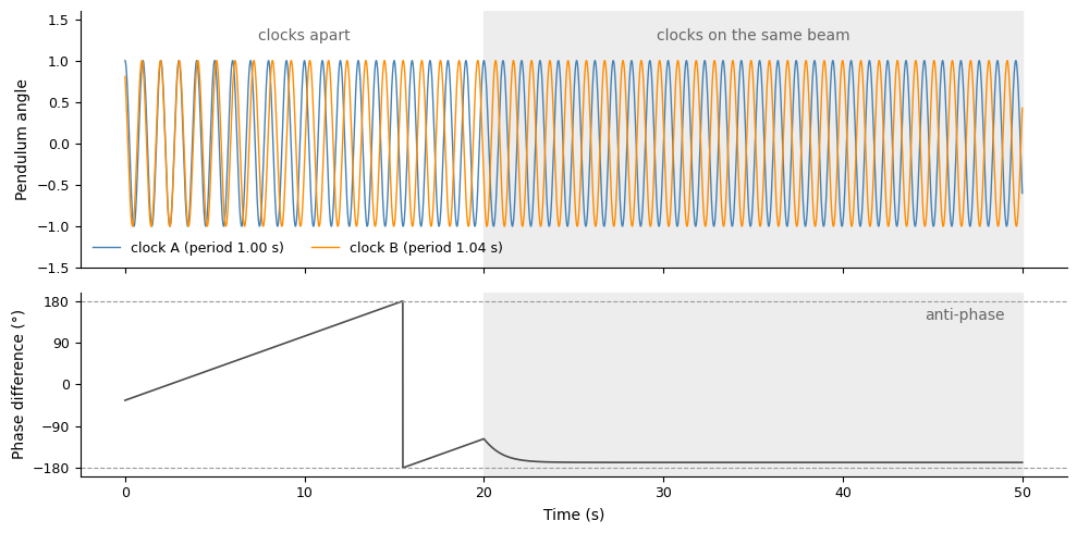
Figure: A simulation of Huygens’s clocks. Two pendulums with periods of 1.00 and 1.04 s drift apart while isolated; their phase difference winds round and round. From 20 s they are weakly coupled through a shared support, and within a few swings they lock into anti-phase, swinging in mirror image.
Measuring entrainment
You can measure your own entrainment with the Tap along app, which scores the mean and spread of your tap timing against a click at any tempo. Most people find that their taps land slightly before the click, by a few tens of milliseconds, which shows that they are predicting the beat rather than reacting to it; the section on producing rhythm in the body explains why. Entrainment can also be read from the whole body. In a motion capture study of people moving to grooves whose beat markers had been shifted by a few tens of milliseconds, the listeners’ movements followed the shifts, without the listeners noticing that anything had changed Danielsen et al., 2015.
Interpersonal synchrony and joint action
Much of this chapter focuses on one person locking attention and movement to an external pulse. Making music together adds coordination between people: ensembles, choirs, and dance partners stabilise a shared tempo, align their movements, and predict each other’s timing. The mechanism is the entrainment described above, now with people coupling to each other as well as to the music. The empirical side of such joint action, from ensemble playing and dance to claims about social bonding, is taken up in the body.
Metre
Metre provides a hierarchical framework for the organisation of rhythm, such as 3/4 or 4/4 metres in music. A metric system typically includes a nested system of pulses at several periodicities, from fast subdivisions to slower bar lengths:
- Beat (pulse/tactus): the fundamental beat we tend to synchronise or entrain to (e.g. the 1–2–3–4 in a 4/4 metre)
- Division levels: subdivisions of the beat (e.g. 8th, 16th, and 32nd notes)
- Multiple levels: slower groupings of the beat (e.g. half-notes and bar-lengths)
Source
import numpy as np
import matplotlib.pyplot as plt
plt.rcParams.update({
    "font.size": 10,
    "axes.titlesize": 11,
    "axes.labelsize": 10,
    "xtick.labelsize": 9,
    "ytick.labelsize": 9,
    "legend.fontsize": 9,
    "figure.figsize": (10, 4),
    "figure.dpi": 100,
    "savefig.dpi": 150,
    "axes.spines.top": False,
    "axes.spines.right": False,
})

levels = [("Bar", 1), ("Half notes", 2), ("Beats (quarter notes)", 4),
          ("Eighth notes", 8), ("Sixteenth notes", 16)]

fig, ax = plt.subplots(figsize=(10, 3.4))
n_levels = len(levels)
ax.axhspan(2.5, 4.6, color="0.93", zorder=0)
ax.axhspan(-0.6, 1.5, color="0.93", zorder=0)
for row, (name, n) in enumerate(levels):
    y = n_levels - 1 - row
    x = np.arange(n) / n
    ax.scatter(x, np.full(n, y), s=260 / (row + 1) + 30, color="steelblue", zorder=3)
    ax.text(-0.04, y, name, ha="right", va="center")
for x in np.arange(0, 1.001, 0.25):
    ax.axvline(x, color="0.8", linewidth=0.8, zorder=1)
ax.axvline(1.0, color="0.4", linewidth=1.5, zorder=2)
ax.text(1.03, 3.55, "Multiple levels\n(groupings of the beat)", va="center", color="0.4")
ax.text(1.03, 2.0, "Beat level\n(what you tap to)", va="center", color="0.4")
ax.text(1.03, 0.45, "Division levels\n(subdivisions of the beat)", va="center", color="0.4")
ax.set_xlim(-0.32, 1.3)
ax.set_ylim(-0.6, 4.6)
ax.set_xticks([0, 0.25, 0.5, 0.75, 1.0])
ax.set_xticklabels(["1", "2", "3", "4", "next bar"])
ax.set_yticks([])
ax.spines["left"].set_visible(False)
ax.set_xlabel("Position in a bar of 4/4")
ax.set_title("Metre as a hierarchy: every level groups or divides the beat level")
plt.tight_layout()
plt.show()
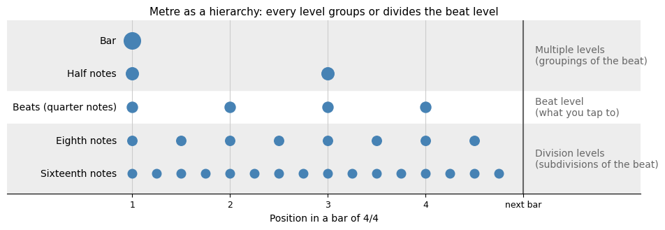
Figure: One bar of 4/4 seen as a stack of pulse levels. Each dot is a pulse; the beat level in the middle is the one listeners usually tap to.
In notation, metre is written as a time signature at the start of the staff. The lower number gives the note value that counts as one pulse and the upper number how many of them make a bar. Beams then show the grouping: 3/4 and 6/8 both hold six eighth notes, but 3/4 beams them in three pairs and 6/8 in two threes, which is exactly the difference between three beats and two. A signature such as 7/8 has beats of unequal length, here 2+2+3, which the section on asymmetric metre below takes up.
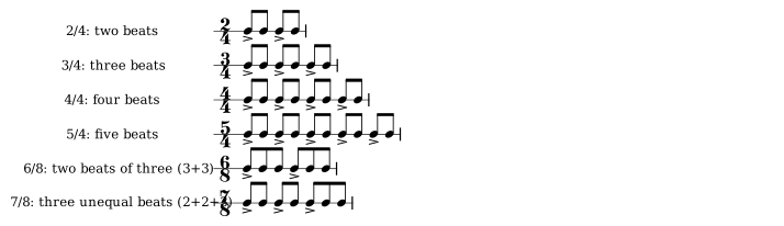
Figure: One bar each of six time signatures on a rhythm staff, drawn to the same scale so that the bars show their relative lengths. The accents mark the beats and the beams show how the pulses are grouped into them.
Subdivision
Subdivisions divide each beat into smaller units. We tend to hear them as subdivisions when their IOI duration is between about 100 and 500 milliseconds. Subdivisions add detail and density, and they often act as stylistic markers (e.g., straight eighths in rock, sixteenths in funk, triplet-based 12/8 in blues).
Drum parts are written on a percussion staff, where the lines and spaces stand for instruments rather than pitches. In the common layout the bass drum sits in the bottom space, the snare in the third space, and the hi-hat (a pair of cymbals on a stand, opened and closed with a foot pedal) above the staff with an x-shaped notehead. The three patterns below differ mainly in their subdivision: eighth notes on the hi-hat in the rock beat, a long–short triplet feel in the 12/8 shuffle, and sixteenths in the funk pattern, while the kick and snare keep their places.
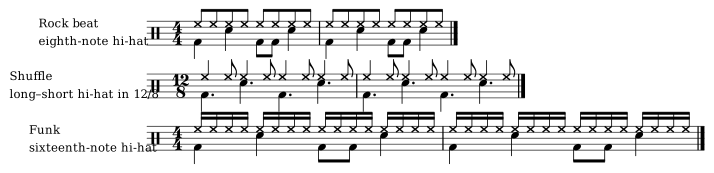
Figure: Three drum patterns on a percussion staff, two bars each, differing in the subdivision of the hi-hat. The bass drum sits in the bottom space, the snare in the third space, and the hi-hat above the staff with an x-shaped notehead. These are the rock, shuffle, and funk presets of the drum machine app.
The Drum machine app lets you hear this directly: one bar of four beats, each divided into two, three, or four steps, on which you draw kick, snare, and hi-hats. Each hit can be soft, medium, or strong, so the grid can also carry a metric accent, the subject of the next section, and a swing control sets the long–short ratio of each pair of subdivisions.
Metric accent
Western music theory traditionally frames metre as a pattern of strong and weak accented beats (e.g., ONE-two-THREE-four in 4/4), with accents thought to align where metrical levels overlap. In practice, this is not always how music is felt or performed. Many groove-based styles emphasise off-beat positions. The downbeat is beat 1 of the bar, an upbeat is the beat or part of a beat that leads into it, and the offbeats are the positions between the beats, such as the “and” in “1-and-2-and”. In popular genres such as rock, soul, and R&B, the snare backbeats on 2 and 4 can feel more salient than beat 1. In reggae, the offbeats on the “ands” may dominate more than the downbeats. Metrical accents, then, are not fixed; practice and cultural convention can redefine them.
Metre as entrainment
Metre can be thought of as entrainment applied to listening. Once a listener has locked on to a beat, attention rises and falls with it, peaking where the next beat is due and dipping in between. It does so at several levels at once, for the subdivision, the beat, and the bar. In this view metre is not a grid printed on the page but a pattern of expectation in the listener, and a metrical accent is simply an event that arrives when attention is at a peak. This is the dynamic attending theory, and the figure below shows the idea.
Source
import numpy as np
import matplotlib.pyplot as plt
plt.rcParams.update({
    "font.size": 10,
    "axes.titlesize": 11,
    "axes.labelsize": 10,
    "xtick.labelsize": 9,
    "ytick.labelsize": 9,
    "legend.fontsize": 9,
    "figure.figsize": (10, 4),
    "figure.dpi": 100,
    "savefig.dpi": 150,
    "axes.spines.top": False,
    "axes.spines.right": False,
})

phi = np.linspace(-0.5, 0.5, 1000)

def attention(period, width):
    """Periodic peaks of attention (a von Mises pulse train) with one peak per period."""
    return np.exp(width * (np.cos(2 * np.pi * phi / period) - 1))

beat = 1.3 * attention(0.25, 12)      # one peak per beat
bar = 1.3 * attention(1.0, 2)         # one broad peak per bar
mixture = beat + bar

fig, ax = plt.subplots(figsize=(10, 3.6))
ax.plot(phi, beat, color="steelblue", linestyle="--", linewidth=1.3, label="Beat level (one peak per beat)")
ax.plot(phi, bar, color="darkorange", linestyle="--", linewidth=1.3, label="Bar level (one peak per bar)")
ax.plot(phi, mixture, color="0.2", linewidth=2, label="Combined metrical expectancy")
ax.text(0, 2.7, "strong beat", ha="center", color="0.3")
for x in (-0.25, 0.25):
    ax.text(x, 1.55, "weak beat", ha="center", color="0.3")
ax.text(-0.09, 2.0, "early", ha="right", color="0.5")
ax.text(0.09, 2.0, "late", ha="left", color="0.5")
ax.set_xlim(-0.5, 0.5)
ax.set_ylim(0, 3.0)
ax.set_xticks([-0.5, -0.25, 0, 0.25, 0.5])
ax.set_xticklabels(["beat 3", "beat 4", "beat 1\n(downbeat)", "beat 2", "beat 3"])
ax.set_xlabel("Position in the bar")
ax.set_ylabel("Expectancy (attention)")
ax.set_title("Dynamic attending: attention peaks at each metrical level add up, so the downbeat is expected most")
ax.legend(loc="upper left")
ax.grid(alpha=0.3)
plt.tight_layout()
plt.show()
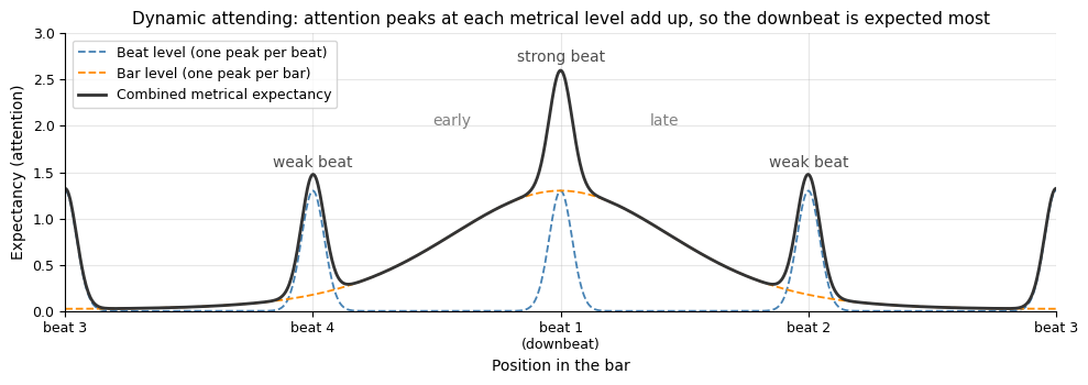
Figure: Two levels of periodic attention and their sum. An event landing inside a tall peak is heard as metrically accented; one landing on a slope is heard as early or late. Schematic, after Large & Palmer (2002).
Think of metrical accent strength as the height and narrowness of an attention peak. Stronger regularity and clearer cueing tighten the window for “on-time”, while looser surfaces widen it without losing the beat. At RITMO, we have done EEG studies that show how the brain prepares its response before an expected beat arrives, both for strictly periodic rhythms and for irregular patterns that are learnable Solli et al., 2025.
Asymmetric metre
Not all metres divide evenly into twos (binary) and threes (tertiary). Asymmetric metres (such as 5/8 or 7/8) have beats of different durations, organised into uneven groupings of equal subdivisions, like 3+2 or 2+2+3. They are common in Balkan, Middle Eastern, and contemporary art-music traditions.
Performers often feel such metres as cycles of unequal steps rather than a uniform grid. The asymmetry can produce a sense of lilt or forward drive distinct from even metres.
The Metre explorer app lets you hear and see this. A cycle of pulses is grouped into beats, from 2/4 to 11/8 and any grouping you type in, drawn as a circle and as a line whose beat lengths show their durations.
Asymmetric metres are one corner of a much larger world of rhythmic patterns that do not fit a grid of equal beats and binary subdivisions. In Norwegian telespringar, for instance, the three beats of the bar are long, medium, and short, a case the chapter returns to at the end.
Dig deeper: rhythmic patterns beyond the even grid
Western notation makes two assumptions that are easy to mistake for facts about rhythm: the beats of a bar are equal, and each beat divides into twos or threes. Many traditions organise time differently, and each of them tells us something about what listeners can entrain to.
Additive metres and aksak. In Bulgarian, Macedonian, Greek, and Turkish dance music, a bar is built by adding short (2) and long (3) units: 7/8 as 2+2+3 (rachenitsa), 9/8 as 2+2+2+3 (daichovo), 11/8 as 2+2+3+2+2 (kopanitsa), and so on up to cycles of 25 pulses in some Turkish usul. The ethnomusicologist Constantin Brăiloiu called this family aksak, Turkish for “limping”. The important perceptual point is that dancers and musicians feel the long and short units as beats, not as groupings of fast pulses. The beat level itself is non-isochronous, with the long beat one and a half times the short one, and people entrain to it without difficulty. London (2012) argues that such metres are well formed precisely because the unequal beats are “maximally even”: the long beats are spread out as far apart as the cycle allows.
Timelines and bell patterns. Much West African and Afro-diasporic music is organised around a short repeating timeline, usually played on a bell or by clapping, against which everything else is heard. The 12-pulse standard pattern (x.x.xx.x.x.x, which has the same interval structure as the Western diatonic scale) and the 16-pulse son clave (x..x..x...x.x...) are the best-known examples, and the tresillo 3+3+2 that runs through so much popular music is the first half of the clave. These patterns are asymmetrical within the cycle, yet they sit inside a regular beat: the standard pattern spans four beats of three pulses each, and its strokes fall on and off the beats in a fixed, learnable way. Which strokes count as “on the beat” can differ between musicians and listeners, which is one reason such music sustains several metric hearings at once.
Euclidean rhythms. Toussaint (2013) noticed that a striking number of traditional timelines are the patterns you get by spreading k onsets as evenly as possible over n pulses, which is exactly what Euclid’s algorithm for the greatest common divisor computes. E(3,8) is the tresillo, E(5,8) the Cuban cinquillo, E(5,12) a common West African and South Indian pattern, and E(7,12) the standard bell pattern. Maximal evenness turns up again here, now at the level of the pattern rather than the beat, which suggests that a shared perceptual constraint underlies very different musical systems. Euclidean rhythm generators are now a standard module in drum machines and modular synthesisers.
Tala. North and South Indian classical music organises time in cycles called tala that can be additive at the beat level as well: jhaptal is 2+3+2+3 (10 beats), rupak 3+2+2 (7), and tintal 4+4+4+4 (16). The first beat of the cycle, sam, is the reference point that soloist and drummer converge on, and cycles can be long enough (and tempos slow enough) that keeping the cycle is a skill in itself. Karnatic konnakol, the spoken syllable system for drumming, lets performers subdivide a beat into fives, sevens, or nines as fluently as Western musicians handle twos and threes.
Non-isochronous subdivision. The unevenness can also sit below the beat. Jazz swing is the familiar case, but it is not the only one. In Malian jembe music the ternary subdivision of a beat is systematically uneven, with the three subpulses taking roughly 40, 30, and 30 percent of the beat rather than a third each, stable across performers and tempos Polak & London, 2014. Like the springar’s unequal beats, this is a timing norm rather than an expressive deviation from a grid. Ensembles play these uneven subdivisions as precisely as even ones Polak et al., 2016, and the way the drummers adapt to each other is spread across musical roles in a pattern that simulations show to be close to optimal for staying together Jacoby et al., 2021. Rainer Polak, who leads this research at RITMO, is extending it to the dancers in the DjembeDance project.
Why this matters for perception. These systems show that entrainment does not require equal beats, only a repeating cycle whose parts are predictable. What varies between traditions is which level carries the unevenness, the subdivision, the beat, or the pattern, and what listeners learn to treat as the reference. Tapping experiments with musicians in Mali, Bulgaria, and Germany make the point directly: everyone shares the simple 1:1 and 2:1 rhythmic prototypes, but prototypes with ratios such as 3:2 and 4:3 appear only in the cultures whose music uses them Polak et al., 2018. Analysis software that quantises everything to a regular grid, or beat trackers trained on isochronous popular music, will misread all of the patterns above, which is a recurring theme when we reach machine listening.
Microrhythm
Microrhythm refers to the fine-scale timing and shaping of events around our subjective reference structures (beat, subdivision). Unlike beat- and subdivision-level rhythms, microrhythm concerns variations in timing at a scale below 100 ms. The ethnomusicologist Charles Keil called such small timing and tuning discrepancies between players participatory discrepancies, arguing that they are what give music its characteristic feel.
At RITMO, many researchers have worked on understanding more about how microrhythm influences music perception and cognition. This has been spearheaded by Anne Danielsen’s work on funk and groove, beginning with her analyses of James Brown and Parliament Danielsen, 2006 and continuing with more fundamental research on microrhythm Danielsen et al., 2024.
Asynchrony and non-isochrony
In terms of timing, we can speak of two related but different forms of microrhythm: asynchrony and non-isochrony. Asynchrony refers to the way musicians can play in a more synchronised (“on-beat”) or asynchronous way (early/“pushed” or late/“laid-back”) relative to one another. Non-isochrony relates to how they might skew the durational ratio of metrical subdivision levels (e.g., 8th or 16th notes) to varying degrees, from isochronous (“straight”) to non-isochronous (“swung”).
Microrhythm can encompass both expressive moment-to-moment nuance and systematic patterns that recur across a piece or style. In many performance traditions, those systematic patterns are the norm, rather than “deviations” from an ideal of perfect metronomic or isochronous timing.
Source
import numpy as np
import matplotlib.pyplot as plt
plt.rcParams.update({
    "font.size": 10,
    "axes.titlesize": 11,
    "axes.labelsize": 10,
    "xtick.labelsize": 9,
    "ytick.labelsize": 9,
    "legend.fontsize": 9,
    "figure.figsize": (10, 4),
    "figure.dpi": 100,
    "savefig.dpi": 150,
    "axes.spines.top": False,
    "axes.spines.right": False,
})

m = 1.0                                   # mean subdivision interval
d = 0.22                                  # displacement
grid = np.arange(5) * m
rows = [
    ("1. Synchronous and isochronous\n(straight)", grid, None),
    ("2a. Asynchronous (late)", grid + d, "+d"),
    ("2b. Asynchronous (early)", grid - d, "-d"),
    ("3. Non-isochronous (swung)", grid + np.array([0, d, 0, d, 0]), "+d"),
]

fig, ax = plt.subplots(figsize=(10, 4.6))
for x in grid:
    ax.axvline(x, color="0.6", linestyle="--", linewidth=1, zorder=0)
for r, (label, times, tag) in enumerate(rows):
    y = len(rows) - 1 - r
    ax.vlines(times, y - 0.3, y + 0.3, color="0.15", linewidth=6)
    ax.text(-0.45, y, label, ha="right", va="center")
    if tag:
        for g, x in zip(grid, times):
            if abs(x - g) > 1e-9:
                ax.annotate("", xy=(x, y + 0.42), xytext=(g, y + 0.42),
                            arrowprops=dict(arrowstyle="->", color="firebrick"))
                ax.text((x + g) / 2, y + 0.5, tag, ha="center", color="firebrick", fontsize=9)
for k in range(4):                                                  # m brackets on top
    ax.annotate("", xy=(grid[k], 3.75), xytext=(grid[k + 1], 3.75),
                arrowprops=dict(arrowstyle="|-|", color="0.35", mutation_scale=3))
    ax.text(grid[k] + m / 2, 3.83, "m", ha="center", color="0.35", style="italic")
for k, label in zip(range(4), ["m + d", "m - d", "m + d", "m - d"]):   # swung durations
    x0 = rows[3][1][k]
    x1 = rows[3][1][k + 1]
    ax.annotate("", xy=(x0, -0.5), xytext=(x1, -0.5),
                arrowprops=dict(arrowstyle="|-|", color="0.35", mutation_scale=3))
    ax.text((x0 + x1) / 2, -0.72, label, ha="center", color="0.35", style="italic", fontsize=9)
ax.set_xlim(-2.9, 4.5)
ax.set_ylim(-0.9, 4.1)
ax.set_yticks([])
ax.set_xticks(grid)
ax.set_xticklabels(["odd\n(beat)", "even", "odd", "even", "odd\n(beat)"])
ax.set_xlabel("Sixteenth-note subdivision positions")
ax.spines["left"].set_visible(False)
ax.set_title("Asynchrony shifts every event against the grid; swing lengthens every other subdivision")
plt.tight_layout()
plt.show()
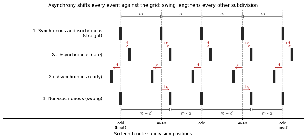
Figure: The reference grid (dashed) has a mean subdivision interval m. Asynchrony displaces events by d in one direction; swing displaces only the even-numbered subdivisions, producing alternating long and short durations. Redrawn after Câmara et al. (2025), Figure 1.
Dig deeper: quantifying asynchrony and swing
Asynchrony is measured as onset displacement (d): how many milliseconds early (negative) or late (positive) an onset falls relative to a timing reference grid. Swing is quantified in two ways: as the absolute onset displacement (d) from the grid position of an even-numbered/off-beat subdivision event, in milliseconds; or as the swing ratio (R) between the duration of an odd-numbered subdivision event (m + d) and the subsequent even subdivision (m − d), where m is the mean inter-onset-interval (IOI) of the subdivision level:
A straight pair gives 1:1 and a triplet-based long–short pair 2:1; the result may also be written as a decimal, such as 1.5.
Beat delay and anticipation
Musicians sometimes play behind or ahead of the beat in a systematic way, whether consciously or not. In rock and soul styles, snare strokes on beats 2 and 4 of a 4/4 metre are often said to be delayed, and in funk, downbeats are said to regularly anticipate “One”. What counts as “late” or “early” always depends on a reference in the given context, whether kick, snare, or the overall grid.
Different degrees of beat delay/anticipation are said to convey different feels. Delayed (late) backbeats in groove styles are often described as “laid-back”: a relaxed feel when only slightly delayed, but a “heavy” or “dragging” feel if delayed too much. Anticipated (early) beats are described as “on-top/pushed”, which at lower magnitudes can sound “snappy” and “driving”, but too much may sound “nervous” or “rushing”.
Source
import numpy as np
import matplotlib.pyplot as plt
plt.rcParams.update({
    "font.size": 10,
    "axes.titlesize": 11,
    "axes.labelsize": 10,
    "xtick.labelsize": 9,
    "ytick.labelsize": 9,
    "legend.fontsize": 9,
    "figure.figsize": (10, 4),
    "figure.dpi": 100,
    "savefig.dpi": 150,
    "axes.spines.top": False,
    "axes.spines.right": False,
})

fig, ax = plt.subplots(figsize=(10, 2.8))
ax.axhline(0, color="0.2", linewidth=1.5)
for x in range(-40, 41, 10):
    ax.plot([x, x], [-0.12, 0.12], color="0.2", linewidth=1.2)
    ax.text(x, 0.2, f"{x:+d}" if x else "0", ha="center", color="0.2")
for x in (-5, 5):
    ax.plot([x, x], [-0.07, 0.07], color="0.2", linewidth=1)
    ax.text(x, 0.2, f"{x:+d}", ha="center", color="0.2", fontsize=8)
labels = [(-30, "nervous"), (-20, "drive"), (-10, "snap"), (1, "groove"),
          (13, "in the pocket"), (27, "dragging")]
for x, name in labels:
    ax.text(x, -0.32, name, ha="center", va="top", color="steelblue", fontweight="bold")
ax.annotate("", xy=(-50, 0), xytext=(-43, 0), arrowprops=dict(arrowstyle="->", color="firebrick"))
ax.text(-46.5, -0.32, "day job", ha="center", va="top", color="firebrick")
ax.annotate("", xy=(50, 0), xytext=(43, 0), arrowprops=dict(arrowstyle="->", color="firebrick"))
ax.text(46.5, -0.32, "get some sleep", ha="center", va="top", color="firebrick")
ax.annotate("", xy=(-22, 0.62), xytext=(-2, 0.62), arrowprops=dict(arrowstyle="->", color="0.4"))
ax.annotate("", xy=(22, 0.62), xytext=(2, 0.62), arrowprops=dict(arrowstyle="->", color="0.4"))
ax.text(-12, 0.7, "on top (early)", ha="center", color="0.4")
ax.text(12, 0.7, "behind (late)", ha="center", color="0.4")
ax.text(0, 0.45, "milliseconds from the beat", ha="center", color="0.4", fontsize=9)
ax.set_xlim(-62, 62)
ax.set_ylim(-0.7, 0.95)
ax.set_axis_off()
ax.set_title("Michael Stewart's \"feel spectrum\" for onset timing at 130 BPM")
plt.tight_layout()
plt.show()
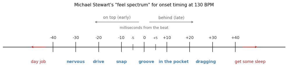
Figure: A producer’s rule of thumb for how far ahead of or behind the beat to place events, and what each amount feels like. Redrawn after Stewart, in Prögler (1995).
Swing
Subdivision notes need not be isochronous (equal), as they are in a straight-8ths hi-hat pattern in rock. Swing, a form of non-isochrony (non-equal durations), describes systematic long–short patterns at the subdivision level.
In jazz, musicians typically do not swing at a perfectly mechanical “triplet swing” ratio of 2:1. Instead, swing ratios in performance can range from close to 1:1 (straight) all the way up to 3:1 (dotted swing) and beyond, depending on tempo, sub-genre, personal style, and other factors. In funk and hip-hop, by contrast, sixteenth notes tend to be swung more subtly (e.g., 1.2:1) unless played in explicit funk-shuffle styles (closer to 2:1, triplet). Swing also depends on tempo. In a study of a samba groove performed at several tempos, the uneven sixteenth notes became more even as the tempo increased, so the same groove has a different swing ratio when played slow and fast Haugen & Danielsen, 2020.
Different swing ratios are thought to impart different degrees of “motional energy” to rhythms. Rhythms with lower swing ratios (closer to 1:1) are described as more “continuous”, “driving”, or “propulsive”, whereas higher swing ratios (up to 2:1 and beyond) tend to give “bounce” or “choppiness”, often accentuating the downbeats and on-beats of the metre.
Perceptual thresholds of microrhythm
Recall from psychoacoustics that the just-noticeable difference (JND) is the smallest change a listener can reliably detect. Microrhythm has its own JNDs, and they are surprisingly small: differences of a few tens of milliseconds are enough to change how a groove feels. How small depends on the sounds involved (sharp drum attacks are easier to judge than blended sustained tones), on tempo and note density, and on musical training.
Dig deeper: measured JND thresholds
Asynchrony JNDs depend strongly on instrument attacks and texture. With overlapping, sustained, or blended tones (e.g., piano, strings, winds, voices), listeners typically need onsets to differ by roughly 20–50 ms before they hear them as asynchronous. In groove contexts, which often involve sharper, more transient sounds (e.g., drums, picked bass), smaller onset displacements can be detected, around 10–20 ms for trained musicians.
For swing, non-musicians tend to need around 30 ms of displacement (a ratio of about 1.4) to hear rhythms as non-straight, while trained musicians can detect swing at around 10 ms displacement (about 1.1–1.2).
For more on JNDs of microrhythm in music, see Câmara et al., 2025.
Groove
Groove can be understood in many ways: as a rhythmic pattern, as a way of playing, and as the pleasurable urge to move that such playing produces. The word has travelled from an LP record’s physical groove to jazz slang and has later also become a research concept Câmara & Danielsen, 2019. Here we focus on groove as “pattern” and as “performance approach”, with an eye on time and rhythm.
As a pattern, a groove can be defined simply as a persistently repeated rhythm, often spanning one or two bars, whose events establish a clear beat and a characteristic subdivision layer. The beat may be externalised (e.g., a kick/snare backbeat in 4/4) or implied by cyclic “isoperiodic” figures that recur predictably. Style identity often hinges on the basic unit (the smallest repeating chunk) and its density referent (the shortest subdivision practically used).
As performance, a groove is the coordinated realisation of that basic unit across parts (e.g., drums, bass, guitar/keys, vocals). Players distribute roles: some layers reinforce the beat (e.g., kicks on beats 1 and 3, snare on 2 and 4), while others supply tension by playing on off-beat subdivisions (e.g., bass accentuating the “2-and”). Grooves often balance stability (an easily entrainable pulse) with off-beat devices that add interest and complexity, such as syncopation and cross-/counter-rhythm (see below).
Syncopation
Syncopation is often described as a local contradiction of a metrical expectation: a note on a weak-position accent, a tie across a strong beat, or the omission of a strong beat followed by sound on a weak one. In 4/4, common cases include stressing the “and” of 2 or 4, tying into 1, or placing a salient event on 3-and while 3 itself is silent. Because the beat is usually firmly established in groove styles, such contradictions tend to add tension without destabilising the metre.
Listening experiments confirm the link to groove: adding syncopation to plain synthesised patterns increases how much listeners want to move, up to a point beyond which the pattern becomes too irregular to follow Sioros et al., 2014.
Counter-/cross-rhythm
When syncopated events recur systematically within the basic unit, they can form larger-scale, patterned off-beat groupings that suggest alternative periodicities to the main beat.
Cross-rhythm (often called “polyrhythm”) occurs when these groupings display a systematic overlap of rhythmic streams whose periodicities (i.e., “metrical levels”) are non-integer multiples. Typical examples in 4/4 are two evenly spaced events over three beats (2:3 cross-rhythms) or four events over three or six beats (4:3 or 4:6 cross-rhythms). The regular pattern of overlapping accents contradicts the beats of the prevailing metre, challenging it and creating greater metrical ambiguity, to the point where one might hear the pulse as either binary or triplet.
Source
import numpy as np
import matplotlib.pyplot as plt
plt.rcParams.update({
    "font.size": 10,
    "axes.titlesize": 11,
    "axes.labelsize": 10,
    "xtick.labelsize": 9,
    "ytick.labelsize": 9,
    "legend.fontsize": 9,
    "figure.figsize": (10, 4),
    "figure.dpi": 100,
    "savefig.dpi": 150,
    "axes.spines.top": False,
    "axes.spines.right": False,
})

def draw(ax, cycle, n_main, n_cross, repeats, title):
    total = cycle * repeats
    main = np.arange(n_main * repeats) * cycle / n_main
    cross = np.arange(n_cross * repeats) * cycle / n_cross
    for r in range(repeats + 1):
        ax.axvline(r * cycle, color="0.5", linewidth=1)
    ax.vlines(main, 0.7, 1.3, color="steelblue", linewidth=8)
    ax.vlines(cross, 1.7, 2.3, color="darkorange", linewidth=8)
    for k, x in enumerate(main):
        ax.text(x, 0.45, str(k % n_main + 1), ha="center", color="steelblue", fontweight="bold")
    for k, x in enumerate(cross):
        ax.text(x, 2.45, str(k % n_cross + 1), ha="center", color="darkorange", fontweight="bold")
    ax.set_xlim(-0.15, total + 0.15)
    ax.set_ylim(0.2, 2.8)
    ax.set_yticks([1, 2])
    ax.set_yticklabels([f"main beat ({n_main} per cycle)", f"cross-rhythm ({n_cross} per cycle)"])
    ax.set_xticks([])
    ax.spines["left"].set_visible(False)
    ax.spines["bottom"].set_visible(False)
    ax.set_title(title, loc="left")

fig, axes = plt.subplots(2, 1, figsize=(10, 4.8))
draw(axes[0], cycle=2, n_main=2, n_cross=3, repeats=2, title="3:2 - three evenly spaced events in the time of two beats")
draw(axes[1], cycle=3, n_main=3, n_cross=4, repeats=2, title="4:3 - four evenly spaced events in the time of three beats")
plt.tight_layout()
plt.show()
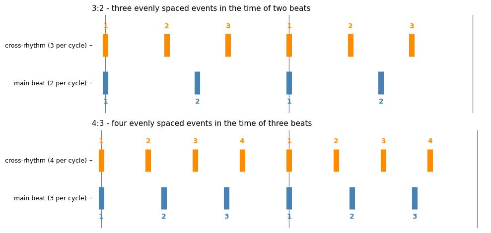
Figure: Cross-rhythms as two simultaneous pulse streams. The two streams meet only at the start of each cycle (vertical lines), which is why they blur the sense of a single pulse.
In most groove styles, though, such overlapping rhythms are usually bounded. They tend to span less than a bar and to coincide again with beat-confirming positions of the metre before repeating. This generates less metrical ambiguity without fundamentally challenging the main pulse. Typical counter-rhythmic groupings in 4/4 are 3+3+2 over eight eighth notes, or 3+3+3+3+2+2 over sixteen sixteenths; listeners may hear secondary “pulses” riding on top of the main metre. The 3+3+2 grouping is the tresillo introduced in the note on rhythmic patterns earlier in this chapter.
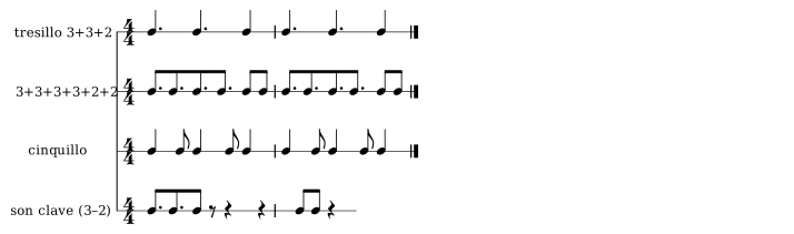
Figure: Four counter-rhythmic patterns written in 4/4. The tresillo and the 3+3+3+3+2+2 grouping are the two mentioned above; the cinquillo and the two-bar son clave are their Afro-Cuban relatives from the note on rhythmic patterns.
A room’s tempo
Everything in this chapter so far has run on musical time scales: onsets tens of milliseconds apart, beats around half a second, phrases lasting a few seconds. However, periodicity can be found everywhere in the world.
Think about the rhythmic nature of many machines. Motors, refrigerators, and ventilation systems all run with different types of duty cycles. A refrigerator typically turns on and off a couple of times per hour. A dishwasher adds a single long phrase with its own internal wash, rinse, and dry structure on top of that pulse.
A critical look: when beats refuse to be equal
Most rhythm research, and most music software, quietly assumes that the beats of a metre are isochronous. For rock, pop, and EDM the assumption mostly holds. Not so much for folk and experimental music.
- The claim under test is that metre rests on equal beats, so that any unevenness is expressive deviation from an underlying regular grid.
- The evidence says otherwise for Norwegian folk music. Measurements of telespringar performances show bars divided into stable long–medium–short beats, in proportions that remain consistent across tunes and performers Haugen, 2016.
- The method combined audio analysis with motion capture of a fiddler and a dancing couple. The fiddler’s foot stamping and the dancers’ vertical motion followed the same non-isochronous pattern, suggesting a shared bodily reference structure rather than sloppy timing.
- The limits are a small number of performers, one regional style, and proportions that vary somewhat between players and districts. The finding does not overturn metre theory; it shows that the reference grid itself can be uneven and learned.
- Fraisse, P. (1982). Rhythm and Tempo. In D. Deutsch (Ed.), The Psychology of Music (pp. 149–180). Academic Press. 10.1016/b978-0-12-213562-0.50010-3
- Snyder, B. (2000). Music and Memory: An Introduction. MIT Press.
- Miller, G. A. (1956). The Magical Number Seven, plus or Minus Two: Some Limits on Our Capacity for Processing Information. Psychological Review, 63(2), 81–97. 10.1037/h0043158
- Koukkari, W. L., & Sothern, R. B. (2006). Introducing Biological Rhythms: A Primer on the Temporal Organization of Life, with Implications for Health, Society, Reproduction, and the Natural Environment. Springer. 10.1007/978-1-4020-4701-5
- Wearden, J. H. (2015). Passage of Time Judgements. Consciousness and Cognition, 38, 165–171. 10.1016/j.concog.2015.06.005
- Allman, M. J., Teki, S., Griffiths, T. D., & Meck, W. H. (2014). Properties of the Internal Clock: First- and Second-Order Principles of Subjective Time. Annual Review of Psychology, 65(1), 743–771. 10.1146/annurev-psych-010213-115117
- Danielsen, A. (Ed.). (2010). Musical Rhythm in the Age of Digital Reproduction. Ashgate. 10.4324/9781315596983
- Clarke, E. F. (1999). Rhythm and Timing in Music. In D. Deutsch (Ed.), The Psychology of Music (2nd ed., pp. 473–500). Academic Press. 10.1016/B978-012213564-4/50014-7
- Nymoen, K., Danielsen, A., & London, J. (2017). Validating Attack Phase Descriptors Obtained by the Timbre Toolbox and MIRtoolbox. Proceedings of the 14th Sound and Music Computing Conference, 214–219.
- Danielsen, A., Nymoen, K., Anderson, E., Câmara, G. S., Langerød, M. T., Thompson, M. R., & London, J. (2019). Where is the beat in that note? Effects of attack, duration, and frequency on the perceived timing of musical and quasi-musical sounds. Journal of Experimental Psychology: Human Perception and Performance, 45(3), 402–418. 10.1037/xhp0000611
- Câmara, G. S., Nymoen, K., Lartillot, O., & Danielsen, A. (2020). Timing Is Everything\ldots Or Is It? Effects of Instructed Timing Style, Reference, and Pattern on Drum Kit Sound in Groove-Based Performance. Music Perception, 38(1), 1–26. 10.1525/mp.2020.38.1.1
- Villing, R. C. (2010). Hearing the Moment: Measures and Models of the Perceptual Centre [Phdthesis, National University of Ireland Maynooth]. https://mural.maynoothuniversity.ie/id/eprint/2284/
- Chafe, C., Cáceres, J.-P., & Gurevich, M. (2010). Effect of Temporal Separation on Synchronization in Rhythmic Performance. Perception, 39(7), 982–992. 10.1068/p6465
- Moelants, D. (2002). Preferred Tempo Reconsidered. Proceedings of the 7th International Conference on Music Perception and Cognition, 580–583.
- Repp, B. H. (2005). Sensorimotor Synchronization: A Review of the Tapping Literature. Psychonomic Bulletin & Review, 12(6), 969–992. 10.3758/BF03206433