This chapter works at the model and interface layers of the five layers. Images are the one medium where the machinery and the surface have to be understood together. A text box is a text box, but an image tool exposes a seed, a guidance number, a step count, and a slot for a reference picture. None of those make sense until you know what the model is doing while it runs.
Image is also the medium where Creative AI announced itself loudest. In 2022 three text-to-image systems reached the public within a few months of each other, and they changed picture-making faster than any tool since the smartphone camera. Designers, illustrators, journalists, lawyers, and the rest of us are still working out what that means.
The aim here is narrower than “learn to prompt an image tool”. It is to give you an accurate account of what happens between the prompt and the picture. Then, when an output is wrong, you can say which knob is wrong, and you can make four images that belong together rather than four images that merely came from the same sentence.
How diffusion works (in pictures)
The image models that reached the public in 2022, and nearly everything built on them since, are diffusion models Ho et al., 2020Rombach et al., 2022. The idea is simpler than it looks.
Source
import numpy as np

import matplotlib.pyplot as plt
plt.rcParams.update({
    "font.size": 10,
    "axes.titlesize": 11,
    "axes.labelsize": 10,
    "xtick.labelsize": 9,
    "ytick.labelsize": 9,
    "legend.fontsize": 9,
    "figure.figsize": (10, 4),
    "figure.dpi": 100,
    "savefig.dpi": 150,
    "axes.spines.top": False,
    "axes.spines.right": False,
})

rng = np.random.default_rng(3)

# A small synthetic "photograph" to push noise into and back out of.
n = 64
yy, xx = np.mgrid[0:n, 0:n] / (n - 1)
red = np.exp(-(((xx - 0.35) ** 2 + (yy - 0.55) ** 2) / 0.05))
green = np.exp(-(((xx - 0.68) ** 2 + (yy - 0.40) ** 2) / 0.04))
image = np.clip(np.stack([0.15 + 0.8 * red, 0.25 + 0.7 * green, 0.35 + 0.5 * yy], -1), 0, 1)
noise = rng.random((n, n, 3))

levels = [0.0, 0.15, 0.35, 0.6, 0.85, 1.0]
frames = [np.clip(np.sqrt(1 - a) * image + np.sqrt(a) * noise, 0, 1) for a in levels]
under = ["image", "+ a bit", "+ more", "noisier", "noisier", "pure noise"]

fig, ax = plt.subplots(figsize=(10, 5))
width, gap = 1.6, 1.95
navy, rose = "#1f2545", "#e8556d"

for i, frame in enumerate(frames):
    x = 0.3 + i * gap
    ax.imshow(frame, extent=[x, x + width, 3.5, 5.1], aspect="auto", zorder=2)
    ax.imshow(frame, extent=[x, x + width, 0.9, 1.9], aspect="auto", zorder=2)
    ax.text(x + width / 2, 3.3, under[i], ha="center", va="top", fontsize=10, color=navy)
    if i < len(frames) - 1:
        ax.annotate("", xy=(x + gap, 4.3), xytext=(x + width, 4.3),
                    arrowprops=dict(arrowstyle="-|>", color=navy, lw=1.8))
        ax.annotate("", xy=(x + width, 1.4), xytext=(x + gap, 1.4),
                    arrowprops=dict(arrowstyle="-|>", color=rose, lw=1.8))

ax.text(0.3, 5.6, "Forward (training): add noise step by step",
        fontsize=11, fontweight="bold", color=navy)
ax.text(0.3, 2.4, "Reverse (inference): denoise from random noise",
        fontsize=11, fontweight="bold", color=rose)
ax.text(1.1, 0.7, "image", ha="center", va="top", fontsize=10, color=navy)
ax.text(11.65 - width / 2, 0.7, "noise", ha="center", va="top", fontsize=10, color=navy)

ax.set_xlim(0, 12)
ax.set_ylim(0.1, 6.0)
ax.axis("off")
plt.tight_layout()
plt.show()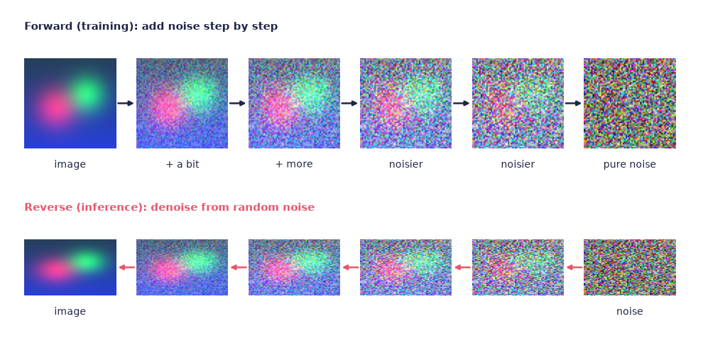
Figure: The top row is forward diffusion, which starts from a real image and adds noise step by step until nothing is left. The bottom row is reverse diffusion, which starts from pure noise and lets a neural network remove it step by step, conditioned on a text prompt.
The training procedure has two halves.
- Forward. Take a real image. Add a tiny bit of noise. Add a tiny bit more. Repeat many times until the image is pure static. Nothing is learned in this half; it is just a recipe for making training pairs.
- Reverse. Train a neural network to undo one step of noise at a time. Given a noisy image and a number saying how noisy it is, predict what was added.
Once the network is trained you can run the reverse half from scratch. Start with pure noise, denoise step by step, and a coherent image emerges out of the static. Nothing was retrieved. The picture is the product of a network that has learned, across many millions of examples, what a slightly less noisy version of any given mess usually looks like.
On its own that gives you a random plausible picture, which is a demonstration rather than a tool. What makes it usable is conditioning, introduced in chapter 2: an extra input fed to the model alongside the noise in order to bias what comes out. For images the most common one is a text prompt, turned into numbers by a text encoder trained to place pictures and their captions near each other in the same space Radford et al., 2021, and injected at every denoising step.
Four practical consequences follow directly from that loop, and between them they cover most of what an image tool offers.
- The model can be reused for image-to-image by starting from a partially noisy version of an existing picture rather than from pure noise. Less added noise means more faithfulness to the input.
- The model can be reused for inpainting by denoising only a masked region and leaving the rest of the pixels alone.
- The model can be reused for outpainting by treating an extension of the canvas as a masked region to be filled.
- The number of steps trades quality against time. Many models released since 2023 produce usable results in four to eight steps using distilled samplers, where the first generation needed fifty.
Latent diffusion Rombach et al., 2022 added the efficiency trick that put these models on ordinary hardware. The denoising does not happen in pixel space, where a single image is millions of numbers, but in a compressed latent space of thousands of numbers. A separate small network encodes into that space and decodes out of it. The picture is only rendered at full resolution at the very end. This is the difference between a model that needs a data centre and a model that runs on a laptop, and it is the main reason open-weight image models exist at all.
Source
from matplotlib.patches import Circle, FancyBboxPatch, Polygon, Rectangle

import matplotlib.pyplot as plt
plt.rcParams.update({
    "font.size": 10,
    "axes.titlesize": 11,
    "axes.labelsize": 10,
    "xtick.labelsize": 9,
    "ytick.labelsize": 9,
    "legend.fontsize": 9,
    "figure.figsize": (10, 4),
    "figure.dpi": 100,
    "savefig.dpi": 150,
    "axes.spines.top": False,
    "axes.spines.right": False,
})

navy, purple, rose = "#1f2545", "#5a2a7a", "#e8556d"

fig, ax = plt.subplots(figsize=(10, 4.4))
ax.set_aspect("equal")


def picture(x, y, size, edge):
    """A picture glyph: a frame holding a sun and two hills."""
    ax.add_patch(Rectangle((x, y), size, size, facecolor="white", edgecolor=edge, linewidth=1.8))
    ax.add_patch(Circle((x + 0.28 * size, y + 0.72 * size), 0.09 * size,
                        facecolor="none", edgecolor=edge, linewidth=1.6))
    ax.add_patch(Polygon([(x + 0.06 * size, y + 0.1 * size), (x + 0.38 * size, y + 0.55 * size),
                          (x + 0.65 * size, y + 0.1 * size)], closed=True,
                         facecolor="none", edgecolor=edge, linewidth=1.6))
    ax.add_patch(Polygon([(x + 0.5 * size, y + 0.1 * size), (x + 0.73 * size, y + 0.42 * size),
                          (x + 0.95 * size, y + 0.1 * size)], closed=True,
                         facecolor="none", edgecolor=edge, linewidth=1.6))


def box(x, y, w, h, text):
    ax.add_patch(FancyBboxPatch((x, y), w, h, boxstyle="round,pad=0.02,rounding_size=0.12",
                                facecolor="#f4f1fa", edgecolor=purple, linewidth=1.8))
    ax.text(x + w / 2, y + h / 2, text, ha="center", va="center", fontsize=11, color=navy)


def arrow(x1, x2, y, colour=navy, style="-|>", dashed=False):
    ax.annotate("", xy=(x2, y), xytext=(x1, y),
                arrowprops=dict(arrowstyle=style, color=colour, lw=1.8,
                                linestyle="--" if dashed else "-"))


picture(0.4, 1.5, 1.7, purple)
ax.text(1.25, 1.25, "millions of numbers", ha="center", va="top", fontsize=10, color=navy)
arrow(2.1, 2.6, 2.35)
box(2.6, 2.0, 1.6, 0.7, "encoder")
arrow(4.2, 4.9, 2.35)

for k in range(3):
    ax.add_patch(Rectangle((4.9 + k * 0.85, 2.0), 0.7, 0.7,
                           facecolor="white", edgecolor=purple, linewidth=1.8))
ax.text(6.0, 2.9, "thousands of numbers", ha="center", va="bottom", fontsize=10, color=navy)
ax.plot([7.3, 7.3, 4.9, 4.9], [2.0, 1.55, 1.55, 2.0], color=rose, lw=1.8, ls="--")
ax.annotate("", xy=(4.9, 2.0), xytext=(4.9, 1.55),
            arrowprops=dict(arrowstyle="-|>", color=rose, lw=1.8))
ax.text(6.1, 1.3, "denoise, step by step, under the prompt",
        ha="center", va="top", fontsize=10, color=rose)

arrow(7.5, 8.0, 2.35)
box(8.0, 2.0, 1.6, 0.7, "decoder")
arrow(9.6, 10.1, 2.35)
picture(10.1, 1.5, 1.7, rose)
ax.text(10.95, 1.25, "rendered once, at the end", ha="center", va="top", fontsize=10, color=navy)

ax.text(1.25, 3.5, "Pixel space", ha="center", fontsize=11, fontweight="bold", color=purple)
ax.text(6.0, 3.5, "Latent space", ha="center", fontsize=11, fontweight="bold", color=purple)
ax.text(10.95, 3.5, "Pixel space", ha="center", fontsize=11, fontweight="bold", color=purple)
ax.text(6.1, 0.35, "The expensive loop runs on the small representation, "
        "which is why these models fit on a laptop.",
        ha="center", fontsize=10, color=navy)

ax.set_xlim(0, 12.2)
ax.set_ylim(0.1, 3.9)
ax.axis("off")
plt.tight_layout()
plt.show()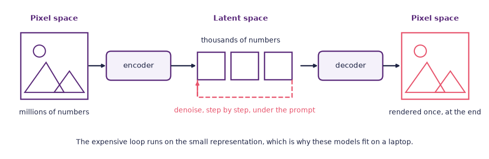
Figure: An encoder compresses the picture into a small latent representation, the denoising loop runs there, and a decoder renders the picture at full resolution only at the end.
The most recent generation of image models uses flow matching or rectified flows rather than plain diffusion Esser et al., 2024. The mathematics is tidier and the sampling is shorter, but the intuition in the figure above still holds: something structureless is pushed, step by step, towards something structured, under the influence of your prompt.
The vocabulary of text-to-image
Every image tool exposes roughly the same small set of knobs, under slightly different names. Learning them once transfers everywhere.
- Prompt. What you want.
- Negative prompt. What you do not want. Often more powerful than people expect, and not supported by every tool.
- Aspect ratio. Square, landscape, portrait. Some compositions work in one and collapse in another, so this is a compositional decision rather than an export setting.
- Guidance, sometimes labelled CFG scale, short for classifier-free guidance. How strictly the model should obey the prompt. Typical defaults sit around five to nine. Higher gives you a more literal reading of your words and often a harsh, oversaturated picture; lower gives you a looser, more varied, sometimes more interesting one.
- Steps. The number of denoising steps. Conventionally a few dozen for a full-quality model and a handful for a distilled one.
- Seed. The random number that generates the starting noise. The same prompt with the same seed in the same model gives you the same image every time, which is what makes controlled comparison possible at all.
- Sampler or scheduler. The algorithm that walks the denoising path. It affects both style and how quickly the image settles.
- Reference image. An extra conditioning input, covered below.
Source
import numpy as np

import matplotlib.pyplot as plt
plt.rcParams.update({
    "font.size": 10,
    "axes.titlesize": 11,
    "axes.labelsize": 10,
    "xtick.labelsize": 9,
    "ytick.labelsize": 9,
    "legend.fontsize": 9,
    "figure.figsize": (10, 4),
    "figure.dpi": 100,
    "savefig.dpi": 150,
    "axes.spines.top": False,
    "axes.spines.right": False,
})

navy, purple, rose = "#1f2545", "#5a2a7a", "#e8556d"

guidance = np.linspace(1, 20, 300)
adherence = 1 - np.exp(-(guidance - 1) / 3.0)
naturalness = 1 / (1 + np.exp((guidance - 9.5) / 2.0))

fig, ax = plt.subplots(figsize=(10, 3.8))
ax.axvspan(5, 10, color="#f4f1fa", zorder=0)
ax.plot(guidance, adherence, color=purple, lw=2.6, label="does it follow the prompt")
ax.plot(guidance, naturalness, color=rose, lw=2.6, label="does it still look natural")

ax.text(7.5, 1.02, "the range most tools default to", ha="center", fontsize=10,
        color=purple)
ax.annotate("the prompt is\npolitely ignored", xy=(1.7, 0.14), xytext=(1.3, 0.66),
            fontsize=10, color="#444444",
            arrowprops=dict(arrowstyle="-|>", color="#8f8a9c", lw=1.2))
ax.annotate("rigid, oversaturated,\nand overcooked", xy=(17.5, 0.14), xytext=(13.4, 0.36),
            fontsize=10, color="#444444",
            arrowprops=dict(arrowstyle="-|>", color="#8f8a9c", lw=1.2))

ax.set_xlim(1, 20)
ax.set_ylim(0, 1.16)
ax.set_xlabel("guidance scale")
ax.set_ylabel("how well it does")
ax.set_yticks([])
ax.legend(loc="center right", frameon=False)
for side in ("right", "top"):
    ax.spines[side].set_visible(False)
ax.text(1.2, -0.24, "a sketch of the trade-off rather than measured values",
        fontsize=9, color="#666666")

plt.tight_layout()
plt.show()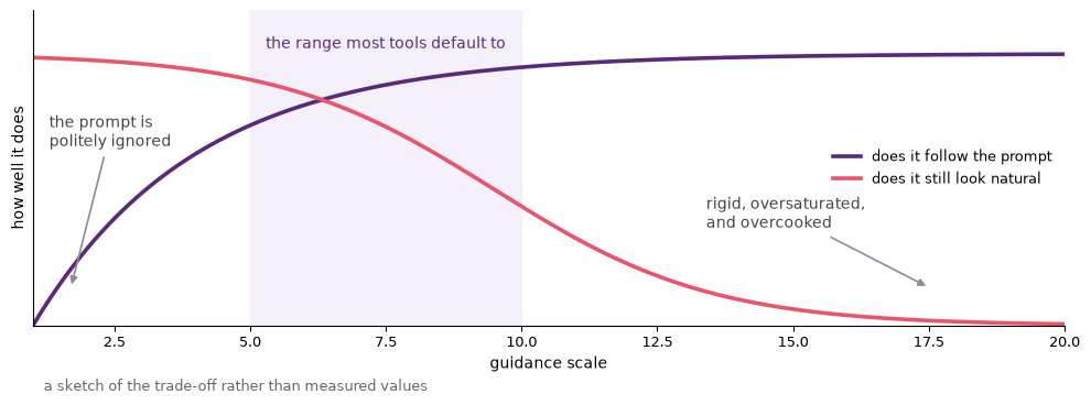
Figure: Raising the guidance scale makes the picture follow the prompt more literally and look less natural, so the useful settings sit where the two curves cross.
Not every tool exposes these controls. Many consumer image services hide the seed, the guidance value, and the step count, so the experiments in this week’s lab cannot be run inside them. A hosted open-weight model, opened as a free demo page in a browser, exposes all three without an installation and without a subscription. Check that a tool shows you a seed field before you choose it for this week.
One discipline matters more than any of the individual settings: change one knob at a time. If you change the prompt and the seed and the guidance, the new picture tells you nothing, because you cannot attribute the difference to anything. That is not a stylistic preference but the only way the tool becomes legible, and it is why the seed is worth more attention than its dull name suggests. A locked seed turns a slot machine into an experiment.
Prompting for images
Image prompts are not language prompts. A language model reads your sentence as instructions; an image model reads it much closer to a bag of weighted concepts, so grammar buys you less and specific nouns buy you more. A working pattern:
[Subject] | [composition] | [style] | [medium] | [lighting] | [mood] | [extra refs]A worked example:
A wooden rowing boat moored at a fjord pier, viewed from a low angle,
black-and-white film photograph, soft early morning light, 50 mm,
nostalgic, in the style of late twentieth-century Scandinavian photography
Four habits do most of the work.
- Be concrete about the subject before you reach for style. “A car” is vague, and vagueness is answered with the average of everything in the training data. “A rusted 1970s estate car parked in front of a yellow wooden house” is something the model can grip.
- Use style words deliberately. Material (oil painting, pen drawing), medium (photograph, render), and period (1970s, Renaissance) each do real work, and they do it more reliably than adjectives like “beautiful” or “high quality”.
- Avoid contradictions. “Photo-realistic illustration in watercolour” asks the model to choose between three things it cannot do at once, and it will choose for you.
- Iterate on what is wrong, not on the whole prompt. If the lighting is off, change only the lighting words. This is the change-one-knob rule applied to the sentence itself.
Negative prompts
Where a tool supports them, negative prompts are where you shut down the failure modes you keep seeing: blurring, extra fingers, watermarks, deformed faces. Treat the negative prompt as a short curated list built from your own failures, not as a copied block of a hundred words. A long negative prompt is mostly superstition, and it costs you conditioning capacity that the positive prompt could be using.
Reference images and control signals
When words run out, show the model what you want. Most tools in use in 2026 accept one or more of the following, which are exactly the conditioning channels from chapter 2 exposed as interface controls.
- A style reference: make it look like this.
- A structural reference: match this composition.
- A pose reference: put the figure in this position.
- A depth or edge map: preserve this geometry, change everything else.
In open-weight tooling these are called ControlNets, small networks trained to inject a spatial signal into the denoiser, and a node-based interface will let you stack several of them at once. Commercial products expose a subset of the same thing under friendlier names such as style reference or character reference.
This is where image generation stops guessing at what you meant and becomes a controllable instrument, and where the honest version of the craft lives. A picture made from your own photograph, your own sketch, and your own depth map is a different artefact from a picture made from a sentence, both aesthetically and ethically. The process memo is where you say which one you made.
Editing instead of generating
For most professional work you will get further by editing an image than by generating one. The same model runs in all of these modes; only the mask and the starting noise change.
- Inpainting. Mask a region and replace it. Swap the object someone is holding, take out a stray sign, repair a mangled hand.
- Outpainting. Extend the canvas beyond its original edges, which is how a portrait crop becomes a banner.
- Variation. The same subject, slightly moved, for choosing between near-identical takes.
- Upscaling. Increase resolution while inventing plausible detail. Note the word inventing: an upscaler does not recover information, it fabricates something consistent with what is there.
- Object removal. A one-click case of inpainting, and the one your phone already does.
Source
import numpy as np
from matplotlib.patches import Rectangle

import matplotlib.pyplot as plt
plt.rcParams.update({
    "font.size": 10,
    "axes.titlesize": 11,
    "axes.labelsize": 10,
    "xtick.labelsize": 9,
    "ytick.labelsize": 9,
    "legend.fontsize": 9,
    "figure.figsize": (10, 4),
    "figure.dpi": 100,
    "savefig.dpi": 150,
    "axes.spines.top": False,
    "axes.spines.right": False,
})

navy, purple, rose = "#1f2545", "#5a2a7a", "#e8556d"
rng = np.random.default_rng(5)

size = 96
ys, xs = np.mgrid[0:size, 0:size]
picture = np.zeros((size, size, 3))
sky = ys / size
picture[..., 0] = 0.36 + 0.5 * sky
picture[..., 1] = 0.42 + 0.44 * sky
picture[..., 2] = 0.62 + 0.32 * sky
sun = (xs - 66) ** 2 + (ys - 70) ** 2 < 11 ** 2
picture[sun] = (0.98, 0.86, 0.55)
for left, width, height, tone in [(6, 16, 40, 0.30), (24, 12, 55, 0.22),
                                  (38, 18, 34, 0.36), (58, 14, 46, 0.26),
                                  (74, 16, 30, 0.33)]:
    picture[0:height, left:left + width] = (tone, tone * 0.9, tone * 1.15)
picture = np.clip(picture, 0, 1)[::-1]

fig, axes = plt.subplots(1, 4, figsize=(10, 3.4))
titles = ["Inpainting", "Outpainting", "Variation", "Upscaling"]
glosses = ["mask a region\nand replace it", "extend past\nthe original edge",
           "the same subject from\na partly noisy copy", "invent detail that\nwas never there"]

axes[0].imshow(picture)
axes[0].add_patch(Rectangle((34, 30), 26, 30, facecolor="white", alpha=0.55,
                            edgecolor=rose, linewidth=2))

pad = 26
wide = np.ones((size + 2 * pad, size + 2 * pad, 3)) * 0.93
wide[pad:pad + size, pad:pad + size] = picture
axes[1].imshow(wide)
axes[1].add_patch(Rectangle((pad, pad), size, size, facecolor="none",
                            edgecolor=rose, linewidth=1.6, linestyle="--"))

noisy = np.clip(picture * 0.65 + rng.normal(0.5, 0.22, picture.shape) * 0.35, 0, 1)
axes[2].imshow(noisy)

blocks = picture.reshape(12, 8, 12, 8, 3).mean(axis=(1, 3))
coarse = np.repeat(np.repeat(blocks, 8, axis=0), 8, axis=1)
combined = coarse.copy()
combined[:, size // 2:] = picture[:, size // 2:]
axes[3].imshow(combined)
axes[3].axvline(size // 2, color=rose, lw=2)
axes[3].text(size * 0.25, 6, "before", ha="center", va="top", fontsize=9,
             color="white")
axes[3].text(size * 0.75, 6, "after", ha="center", va="top", fontsize=9,
             color="white")

for ax, title, gloss in zip(axes, titles, glosses):
    ax.set_xticks([])
    ax.set_yticks([])
    ax.set_title(title, fontweight="bold", color=purple, pad=8)
    ax.set_xlabel(gloss, color="#444444", labelpad=6)
    for side in ax.spines.values():
        side.set_visible(False)

plt.tight_layout()
plt.show()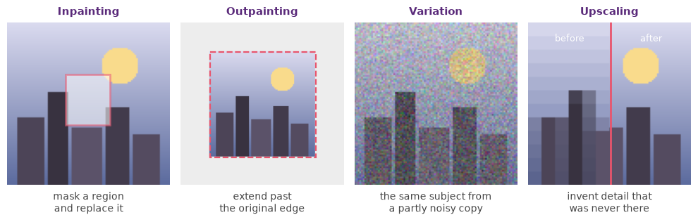
Figure: Four editing modes running on the same picture, and in every one of them the model is asked to fill a gap that you defined rather than to invent a whole image.
Editing keeps you closer to authorship, because the thing being changed is something you chose or made. It is also the workflow most likely to survive whatever the tools look like in five years, since the underlying operation, mask and regenerate, has been stable since 2022.
Consistency across a series
A single striking image is easy. Getting four images to show the same character, place, or object is the problem that separates a demonstration from a piece of work, and it is where most student projects run into trouble. The reason is structural: the seed sets the noise, the prompt sets the concepts, and nothing in either of them is an identity. Ask twice for “the same woman” and you get two women who match the description.
Three tools address this, in ascending order of effort.
Character reference images condition the generation on a picture of the subject, so the model is matching an appearance rather than reconstructing one from words. This is the right tool when you have one good image of the subject and need three or four more of it, and when close enough is good enough. It is the cheapest option, it needs no training, and it drifts under large changes of pose or lighting, because the model is being asked to generalise from a single view.
Seed locking holds the noise fixed and changes only the prompt, so the composition, palette, and lighting stay put while the content shifts. This is the right tool when what you need to hold constant is the frame rather than the subject: the same street in four seasons, the same room at four times of day. It gives you a visually coherent set almost for free. It will not keep a face the same, because a face is content, not framing.
Source
import numpy as np
from matplotlib.patches import Ellipse

import matplotlib.pyplot as plt
plt.rcParams.update({
    "font.size": 10,
    "axes.titlesize": 11,
    "axes.labelsize": 10,
    "xtick.labelsize": 9,
    "ytick.labelsize": 9,
    "legend.fontsize": 9,
    "figure.figsize": (10, 4),
    "figure.dpi": 100,
    "savefig.dpi": 150,
    "axes.spines.top": False,
    "axes.spines.right": False,
})

navy, purple, rose = "#1f2545", "#5a2a7a", "#e8556d"

seeds = [11, 12, 13]
prompts = [("in autumn", ["#f6efe2", "#c88a3d", "#8f5b2a", "#5d4326"]),
           ("at night", ["#1f2545", "#3d3f6b", "#5a2a7a", "#8f8ac4"]),
           ("in snow", ["#f2f5fa", "#b9c8dc", "#7d94b4", "#4a5a72"])]

fig, axes = plt.subplots(len(seeds), len(prompts), figsize=(10, 4.4))

for row, seed in enumerate(seeds):
    rng = np.random.default_rng(seed)
    shapes = [(rng.uniform(0.15, 0.85), rng.uniform(0.15, 0.85),
               rng.uniform(0.2, 0.55), rng.uniform(0.2, 0.55),
               rng.integers(1, 4)) for _ in range(5)]
    for column, (prompt, palette) in enumerate(prompts):
        ax = axes[row, column]
        ax.set_facecolor(palette[0])
        for x, y, width, height, tone in shapes:
            ax.add_patch(Ellipse((x, y), width, height,
                                 facecolor=palette[int(tone)], edgecolor="none",
                                 alpha=0.85))
        ax.set_xlim(0, 1)
        ax.set_ylim(0, 1)
        ax.set_xticks([])
        ax.set_yticks([])
        for side in ax.spines.values():
            side.set_visible(True)
            side.set_color("#cfc7dd")
        if row == 0:
            ax.set_title(prompt, color=purple, fontweight="bold", pad=8)
        if column == 0:
            ax.set_ylabel(f"seed {seed}", color=navy, labelpad=8)

fig.text(0.5, 0.015, "the seed fixes the arrangement along a row, and the prompt "
         "changes what fills it", ha="center", fontsize=10, color=navy)
plt.tight_layout(rect=(0, 0.05, 1, 1))
plt.show()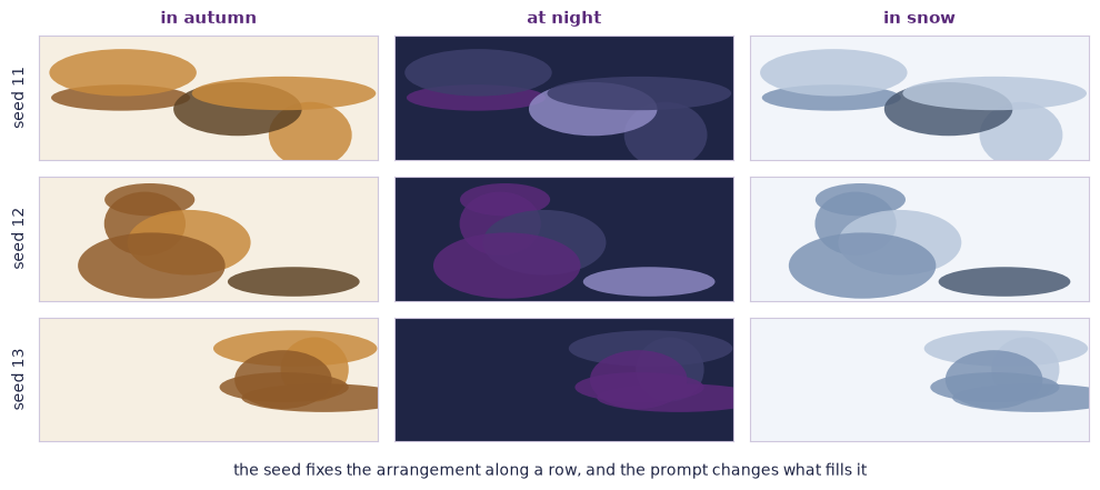
Figure: Nine sketches in which the seed is held along each row and the prompt changes along each column, so the arrangement stays put while the palette moves.
LoRA fine-tunes, where LoRA is short for low-rank adaptation, take a small number of images of your subject, typically in the tens, and train a small set of extra weights that ride on top of a frozen open-weight model. The subject becomes a word the model knows. This is the right tool when the same character has to appear across many images over weeks, which is why it is standard practice in comics, animation, and brand work. It is also the only one of the three that genuinely learns your subject. It costs you an open-weight model, a training run, and a rights question, since those training images have to be yours to use.
For a four-image series made in a 90-minute lab, seed locking plus a character reference will get you most of the way. Reach for a fine-tune only when the series outlives the week.
Where image models still struggle
The failure list has been shrinking every year, so read this as a snapshot of early 2026 rather than a permanent limit.
- Hands, feet, jewellery, and complicated logos. Anything with a strict internal count or structure that the training data mostly shows in passing.
- Faithful portraits of named individuals. Technically difficult and, in most commercial tools, deliberately restricted.
- Multi-step composition. “A man holds a cat in one hand and points with the other at a sign reading Open” asks for several spatial relations at once, and models reliably drop one.
- Text inside pictures. Much improved since 2023 and still not solved, especially for anything longer than a few words or in a language other than English.
- Diagrams and infographics. A model can produce something with the exact visual grammar of a chart and no relationship at all to any data. This failure is unusually dangerous because the output looks authoritative.
- Anything requiring a count. Five chairs is a request the model treats as a suggestion.
The pattern is worth naming, because it predicts the next failure you meet. These models are excellent at texture and plausibility and weak at discrete structure. Wherever a correct answer depends on counting, spelling, or a fact rather than on looking right, expect to check it yourself.
Dig deeper: generating locally
Everything in this chapter can be done in a browser. Running a model on your own machine is what lets you fix the seed with confidence, batch a hundred variations overnight, and keep working when a service changes its terms. It is also the only way to use a fine-tune you trained yourself.
The diffusers library is the standard route Hugging Face, 2024. The listing below is not executed when this book is built, because it needs a GPU and a model download of several gigabytes. Install the diffusers, transformers, and torch packages, and it runs as it stands.
import torch
from diffusers import StableDiffusionPipeline

pipe = StableDiffusionPipeline.from_pretrained(
    "stabilityai/sd-turbo",
    torch_dtype=torch.float16,
).to("cuda")  # or "mps" on a recent Mac, or "cpu" if you are patient

generator = torch.Generator(device="cuda").manual_seed(42)

img = pipe(
    "a wooden rowing boat at sunrise on a fjord, watercolour",
    num_inference_steps=4,
    guidance_scale=1.0,
    generator=generator,
).images[0]
img.save("boat.png")
Two things to notice. The generator line is seed locking made explicit: pass the same number and you get the same picture back, which is what makes the grids in this week’s lab into an experiment rather than a collection. And num_inference_steps=4 is only sane because this is a distilled model; on a full model the same value gives you noise with ambitions.
This week’s lab: Explore, Reflect, Create
This lab has three movements: find out what each knob does, argue about what the model leaves out, and make something you would put your name on.
Explore (about 30 min)
A controlled experiment. Work in a tool that shows you the seed, the guidance value, and the step count, since a service that hides its settings cannot answer any of the questions below. Write one base prompt with a clear subject, composition, and style, and keep it fixed for the whole exercise.
- Generate four images with the same prompt and the same seed at four different aspect ratios.
- Generate four with the same prompt and the same seed at four different guidance values, for example 3, 6, 9, and 12.
- Generate four with the same prompt and four different seeds, changing nothing else.
- Generate four in which the prompt is unchanged except for the lighting words.
Lay each set out as a labelled grid, so you leave the lab with four grids rather than sixteen loose files. Then answer one question in a sentence: which knob mattered most for your subject, and why that subject rather than another.
Image-to-image. Take a photograph you have the rights to, your own if possible, and run it through an image-to-image pipeline at three denoise strengths, around 0.3, 0.5, and 0.8. Put the three outputs next to the original and mark where on the axis from fidelity to freedom you would want to sit for a real job.
One more generation, for the next block. Generate a single image of “a typical Norwegian street”, and find a photograph of an actual Norwegian street to put beside it, ideally one you took yourself. Bring both to the Reflect round.
Optional. Compare your best and worst grid in the Seed and guidance grid viewer.
Reflect (about 15 min)
Work in pairs, then in plenary. This is a discussion, not a writing block.
- Put your “typical Norwegian street” generation beside the photograph you brought. Ask your partner what has been averaged away: which decade, which weather, which parts of the country, which people, which mess. Be specific, because “it looks generic” is the answer that stops the conversation rather than starting it.
- Ask each other where the averaging would matter in your own discipline, and where it would not. If you study people, name what the averaged image most resembles: a category, a stereotype, or the picture somebody would draw from memory.
- Close the round by stating aloud the series you are going to make in the Create block: the subject, the through-line, and which of the three consistency tools you will use.
Create (about 45 min)
Assemble one finished piece from what you generated above. This is a portfolio artefact, not an exercise. Choose one form:
- a four-image series with a shared subject and a clear conceptual through-line, for example the same Oslo street in four seasons;
- a single poster combining one of your generations with typography you set yourself;
- a photograph and redraw diptych that puts a real image next to its image-to-image variant and lets the viewer see both.
Whichever you choose, write a 100-word honest caption recording the tool, the model, the seed where you can see it, the prompt, the variations you tried, and every human edit. The caption is part of the artefact, not metadata about it, and a series that needs the caption hidden is not finished.
A2 is due this week. AI-assisted text in your discipline was set in week 4 and is handed in now, so keep an hour clear for it; the image series is a separate portfolio piece and does not replace it.
Optional, for the commons. If one of your photographs would genuinely help explain something, for example a street in a place Wikipedia has no picture of, upload it to Wikimedia Commons. Commons accepts AI-generated images only when they have a realistic educational use, such as showing what a diffusion model does with a given prompt, and they must be labelled as generated. Your own photograph is usually the more useful contribution.
At home, write this week’s entry in your practice log using the practice log template.
A critical look: does an image model copy its training images?
The claim. A diffusion model is a collage machine. It has stored the pictures it was trained on and reassembles fragments of them on request, so every output is a copy of somebody’s work and the only question is how well hidden the seams are.
The evidence. There is real evidence for a narrow version of this. In 2023 two research groups showed that training images can be pulled back out of a diffusion model. One team recovered around a hundred near-duplicates of specific training images from the open image model alone. It did so by generating on the order of a hundred million pictures from hundreds of thousands of prompts aimed at candidates it had already identified Carlini et al., 2023. Another found copied content in a small percentage of outputs from a widely used open model and traced it to the same cause Somepalli et al., 2023. Both point at the same mechanism. The images that come back are overwhelmingly ones that appeared many times in the training set, whether as a stock photo reused across thousands of pages or a famous painting reproduced everywhere. Duplication in the data is what turns a general pattern into a memorised instance.
The method. Look at how those findings were produced, because the two studies were built to answer different questions. The extraction team Carlini et al., 2023 started from candidate images already known to be duplicated in the training set, wrote prompts aimed straight at them, generated many samples per prompt, and ran a nearest-neighbour search against the training data to find matches. That is an adversarial extraction attack, and it is the right design for its question, which is can a copy be forced out at all. It is the wrong design for the question people quote it for, which is how often does this happen in ordinary use, because a procedure built to maximise a rate cannot also measure it. The replication study Somepalli et al., 2023 asked that second question instead, sampling generations without aiming at known duplicates and then retrieving the nearest training images to estimate how often a near match turns up unprompted. Read together they say that copies can be extracted deliberately and that they surface rarely otherwise, and neither figure substitutes for the other.
The limits. So memorisation is real, rare, and concentrated on images the training set contained many times over. For the overwhelming majority of outputs, “copy” is simply the wrong word: a model of a few gigabytes cannot be storing the billions of images it saw, and what it holds is a set of statistical regularities, not an archive. The rare exact copy is the exception that shows the rule, since a system built as what chapter 3 calls an anarchive of relations will occasionally return a record anyway. That is why the duty to record provenance falls on the maker rather than on the model. But this does not settle the ethics. The cases filed from 2023 onwards, among them Andersen v. Stability AI United States District Court, Northern District of California, 2023 and Getty Images v. Stability AI High Court of Justice (UK),US District Court, District of Delaware, 2023, mostly turn on whether training on scraped images was lawful, not on whether outputs are copies. A model that never reproduces a single training image still learned everything it knows from work that was taken without asking. That chapter sets out the argument and where the law had reached by 2026. The technical answer to “is it a collage” is no. The answer to “is it fair” is not a technical question.
- Ho, J., Jain, A., & Abbeel, P. (2020). Denoising Diffusion Probabilistic Models. Advances in Neural Information Processing Systems (NeurIPS). https://arxiv.org/abs/2006.11239
- Rombach, R., Blattmann, A., Lorenz, D., Esser, P., & Ommer, B. (2022). High-Resolution Image Synthesis with Latent Diffusion Models. IEEE/CVF Conference on Computer Vision and Pattern Recognition (CVPR). https://arxiv.org/abs/2112.10752
- Radford, A., Kim, J. W., Hallacy, C., Ramesh, A., Goh, G., Agarwal, S., Sastry, G., Askell, A., Mishkin, P., Clark, J., Krueger, G., & Sutskever, I. (2021). Learning Transferable Visual Models From Natural Language Supervision. International Conference on Machine Learning (ICML). https://arxiv.org/abs/2103.00020
- Esser, P., Kulal, S., Blattmann, A., Entezari, R., Müller, J., Saini, H., Levi, Y., Lorenz, D., Sauer, A., Boesel, F., Podell, D., Dockhorn, T., English, Z., Lacey, K., Goodwin, A., Marek, Y., & Rombach, R. (2024). Scaling Rectified Flow Transformers for High-Resolution Image Synthesis. https://arxiv.org/abs/2403.03206
- Hugging Face. (2024). Diffusers — State-of-the-art Diffusion Models for Image, Video, and Audio Generation. Hugging Face. https://huggingface.co/docs/diffusers/index
- fourMs Lab. (2026). Musical Gestures Toolbox for Python. https://github.com/fourMs/MGT-python
- Carlini, N., Hayes, J., Nasr, M., Jagielski, M., Sehwag, V., Tramèr, F., Balle, B., Ippolito, D., & Wallace, E. (2023). Extracting training data from diffusion models. 32nd USENIX Security Symposium. https://arxiv.org/abs/2301.13188
- Somepalli, G., Singla, V., Goldblum, M., Geiping, J., & Goldstein, T. (2023). Diffusion art or digital forgery? Investigating data replication in diffusion models. Proceedings of the IEEE/CVF Conference on Computer Vision and Pattern Recognition. https://arxiv.org/abs/2212.03860
- Andersen v.\ Stability AI Ltd. (2023). United States District Court, Northern District of California. https://www.theverge.com/2024/8/13/24219520/ai-art-copyright-lawsuit-stability-midjourney-deviantart-runway
- Getty Images v.\ Stability AI. (2023). High Court of Justice (UK). https://www.theverge.com/2023/2/6/23587393/ai-art-copyright-lawsuit-getty-images-stable-diffusion
- Gatys, L. A., Ecker, A. S., & Bethge, M. (2015). A Neural Algorithm of Artistic Style. https://arxiv.org/abs/1508.06576
- Manovich, L. (2018). AI Aesthetics. Strelka Press. http://manovich.net/index.php/projects/ai-aesthetics
- Hertzmann, A. (2018). Can Computers Create Art? Arts, 7(2), 18. 10.3390/arts7020018