This chapter works at the data and model layers of the five layers. It is the one chapter in the book that is mostly about machinery. Everything after it is about what you do with the machinery, and almost every argument you will meet in those chapters, about quality, bias, authorship, or cost, turns out to depend on something in here.
You do not need the equations. What you need is a mental model: the cast of characters, and the single shift that turned a back-office technology into a creative instrument. By the end of the chapter you should be able to explain over coffee, in plain language, what happens when somebody says “we trained a model on a billion images and now we are using it to generate logos”. You should also be able to say precisely which part of that sentence to be suspicious of.
Learning from examples
Imagine you want to teach a computer to tell cats from dogs in photographs. You have two strategies.
- Write rules by hand. “If the ears are pointy and the snout is narrow, then it is a cat.” This is the symbolic AI of the mid-twentieth century. It works for small, tidy problems and it breaks for anything visual at the level of the real world, because you cannot enumerate the ways a cat can be lit, posed, cropped, or half hidden behind a chair.
- Show it many examples of cats and dogs labelled as such, and let it learn the rule itself. This is machine learning.
The second strategy won, and it won so completely that the phrase “AI” now nearly always means the second one. The reason is not that rules are stupid, but that the world has more exceptions than any team of rule writers can keep up with, and examples are cheap while rules are expensive.
Source
from matplotlib.patches import FancyBboxPatch

import matplotlib.pyplot as plt
plt.rcParams.update({
    "font.size": 10,
    "axes.titlesize": 11,
    "axes.labelsize": 10,
    "xtick.labelsize": 9,
    "ytick.labelsize": 9,
    "legend.fontsize": 9,
    "figure.figsize": (10, 4),
    "figure.dpi": 100,
    "savefig.dpi": 150,
    "axes.spines.top": False,
    "axes.spines.right": False,
})

navy, purple, rose = "#1f2545", "#5a2a7a", "#e8556d"

fig, ax = plt.subplots(figsize=(10, 3.2))


def box(x, w, title, subtitle=None):
    ax.add_patch(FancyBboxPatch((x, 1.6), w, 1.0,
                                boxstyle="round,pad=0.02,rounding_size=0.15",
                                facecolor="#f4f1fa", edgecolor=purple, linewidth=2))
    ax.text(x + w / 2, 2.22 if subtitle else 2.1, title, ha="center", va="center",
            fontsize=11, fontweight="bold", color=navy)
    if subtitle:
        ax.text(x + w / 2, 1.92, subtitle, ha="center", va="center",
                fontsize=10, color="#444444")


box(0.4, 1.8, "Data")
box(3.0, 2.4, "Model", "(parameters)")
box(6.2, 2.4, "Prediction")
box(9.4, 1.6, "Loss")

for x1, x2 in [(2.2, 3.0), (5.4, 6.2), (8.6, 9.4)]:
    ax.annotate("", xy=(x2, 2.1), xytext=(x1, 2.1),
                arrowprops=dict(arrowstyle="-|>", color=navy, lw=2))

ax.annotate("", xy=(4.2, 2.6), xytext=(10.2, 2.6),
            arrowprops=dict(arrowstyle="-|>", color=rose, lw=2, linestyle="--",
                            connectionstyle="arc3,rad=0.35"))
ax.text(7.2, 4.0, "update parameters to reduce loss",
        ha="center", fontsize=11, color=rose)

ax.set_xlim(0, 11.4)
ax.set_ylim(1.2, 4.3)
ax.axis("off")
plt.tight_layout()
plt.show()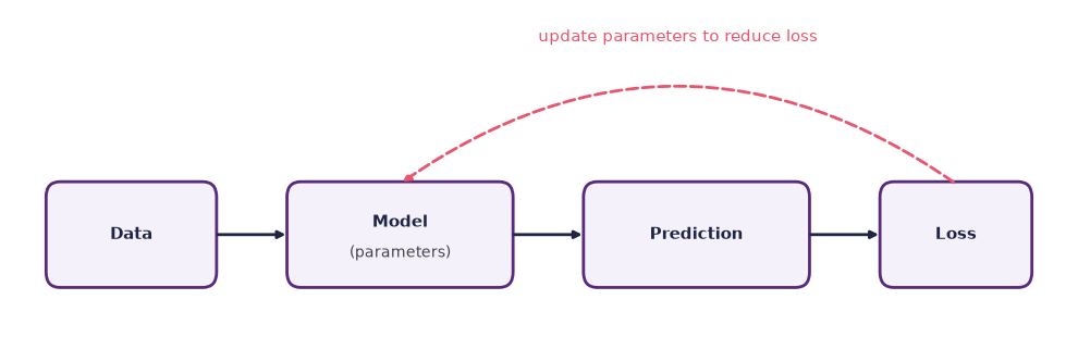
Figure: A simple machine-learning pipeline. Data flows into a model with parameters, the model produces a prediction, and a loss measures how wrong the prediction is and is used to update the parameters.
The diagram above is essentially the whole field. What the data looks like, what shape the model takes, and how the loss is measured all change wildly between applications, and those differences fill the research literature. But the loop is always the same, and it is worth carrying that loop in your head as a single picture.
Six words do most of the work in this chapter. Learn them here and the rest of the book becomes readable.
Data
Data is the fuel. Every model you will use in this course was trained on a dataset, and the shape of that dataset is the single best predictor of what the model will be good at.
- Images and AI: public photography, large open image and caption collections scraped from the web, licensed stock libraries, museum archives.
- Text: books, encyclopedias, web crawls of the open internet, scientific papers, code repositories, forum posts.
- Audio: music libraries, podcasts, speech corpora, video platform soundtracks.
- Video and AI: public video platforms, licensed footage libraries, motion-capture archives.
Two properties of a dataset matter more than its size: its content, meaning what is in it and in what proportion, and its consent, meaning whether the people who made the material agreed to this use. Neither property is visible in a demonstration, though both determine what you get.
Chapter 3 returns to consent, labour, and licensing as an ethical and legal question.
Models
A model is a function with parameters. In modern AI the function is a neural network: a layered chain of multiplications, additions, and simple non-linear operations. The parameters are the numbers, often billions of them, that determine which input produces which output.
You do not need to know the inner workings to use a model, just as you do not need to know how a violin is made to play one. Two facts, though, do matter.
- The function is differentiable. For every parameter, you can compute which direction would make the prediction slightly better. That is the whole reason training is possible at all.
- The function is huge. Models in use in 2026 range from a few hundred million to a few trillion parameters, and the model file alone can run to tens of gigabytes. Size is why these systems live in data centres rather than on your laptop, and it is why running them costs money and energy.
Training
Training is the process of repeatedly
- taking a batch of examples from the dataset,
- making predictions with the current parameters,
- measuring the loss, a single number saying how wrong the predictions were, and
- nudging every parameter a little in the direction that reduces the loss.
That is it. There is no fifth step where understanding is inserted. The loop runs billions of times for a large model, typically for weeks on hundreds or thousands of specialised processors, and it consumes a great deal of electricity. Strubell and colleagues estimated the carbon cost of training a large language model already in 2019, and the models have grown by orders of magnitude since Strubell et al., 2019.
The result of training is a trained model: the network plus one specific set of parameter values. That file is the artefact that is shipped, sold, licensed, or leaked.
Inference
Inference is what happens when you use a trained model. You feed it an input, a prompt, an image, an audio clip, and it produces an output. Inference is far cheaper than training, fractions of a cent rather than millions, but at the scale of hundreds of millions of daily users it adds up to a comparable amount of energy over a model’s lifetime.
When you type into a chat assistant, you are running inference on a model that was trained months earlier. The model’s parameters do not change while you use it. It does not learn from you.
This distinction resolves a surprising number of confusions. “The AI learned my style” is, in nearly every consumer tool, false in the training sense and true only in the sense that your examples sat in the input window during one session.
Generalisation
The aim is a model that does well on new examples it has never seen, and that ability is called generalisation. Its opposite is overfitting: the model has effectively memorised the training examples and does poorly on anything else.
Generalisation is why a face-recognition system can recognise a face that was never in its training set, and why a language model can write a paragraph about a topic invented after it was built. It is also, as later chapters show, exactly why such a paragraph can be fluent and subtly wrong.
Bias
Models inherit the bias of their data. If a dataset over-represents English-speaking, Western, web-published, well-photographed material, the model will be best at exactly that material and blandest everywhere else.
This is worth stating carefully, because it is often misread as an accusation of bad intent. Bias here is a property of the data, propagated by an averaging process that is working correctly. A model trained to predict what is typical of its dataset will reproduce whatever that dataset makes typical, including who appears in it, who is described how, and which languages, bodies, and places are well covered Bender et al., 2021Crawford, 2021. You cannot debug it out of the model without changing the data or the objective. Chapter 3 takes up what follows from that, ethically and practically; for now, treat every output as a sample from somebody’s archive rather than from the world.
From networks to generators
A very short tour of neural networks
A neural network is a stack of layers. Each layer takes a list of numbers, multiplies them by another list of numbers (the parameters), adds a small offset, and passes the result through a simple non-linear function. Stack that operation many times and you get something flexible enough to model very complex patterns Goodfellow et al., 2016.
Source
from matplotlib.patches import Circle

import matplotlib.pyplot as plt
plt.rcParams.update({
    "font.size": 10,
    "axes.titlesize": 11,
    "axes.labelsize": 10,
    "xtick.labelsize": 9,
    "ytick.labelsize": 9,
    "legend.fontsize": 9,
    "figure.figsize": (10, 4),
    "figure.dpi": 100,
    "savefig.dpi": 150,
    "axes.spines.top": False,
    "axes.spines.right": False,
})

navy, purple, rose = "#1f2545", "#5a2a7a", "#e8556d"

fig, (unit, net) = plt.subplots(1, 2, figsize=(10, 3.8),
                                gridspec_kw={"width_ratios": [1, 1.25]})
for ax in (unit, net):
    ax.axis("off")

unit.set_title("One unit", fontweight="bold", color=purple, pad=12)
inputs = [(0.7, 2.9), (0.7, 2.0), (0.7, 1.1)]
for index, (x, y) in enumerate(inputs):
    unit.add_patch(Circle((x, y), 0.22, facecolor="#f4f1fa", edgecolor=purple, lw=1.6))
    unit.text(x - 0.45, y, f"in {index + 1}", ha="right", va="center",
              fontsize=10, color=navy)
    unit.annotate("", xy=(2.35, 2.0), xytext=(x + 0.24, y),
                  arrowprops=dict(arrowstyle="-|>", color="#8f8a9c", lw=1.4))
    unit.text((x + 2.3) / 2, (y + 2.0) / 2 + (0.16 if y > 2 else -0.2),
              f"weight {index + 1}", ha="center", fontsize=9, color="#666666")

unit.add_patch(Circle((2.7, 2.0), 0.62, facecolor=purple, edgecolor=purple, lw=1.6))
unit.text(2.7, 2.16, "add", ha="center", va="center", fontsize=11,
          color="white", fontweight="bold")
unit.text(2.7, 1.85, "then bend", ha="center", va="center", fontsize=9, color="#e6dff0")
unit.annotate("", xy=(4.15, 2.0), xytext=(3.35, 2.0),
              arrowprops=dict(arrowstyle="-|>", color=navy, lw=1.8))
unit.text(4.3, 2.0, "out", ha="left", va="center", fontsize=10, color=navy)
unit.text(2.4, 0.35, "the weights and the offset are the parameters",
          ha="center", fontsize=10, color="#444444")
unit.set_xlim(0, 5.2)
unit.set_ylim(0.1, 3.6)

net.set_title("A small network", fontweight="bold", color=purple, pad=12)
layers = [3, 5, 5, 2]
labels = ["input", "hidden", "hidden", "output"]
positions = []
for index, count in enumerate(layers):
    x = 0.8 + index * 1.55
    ys = [2.0 + (position - (count - 1) / 2) * 0.62 for position in range(count)]
    positions.append([(x, y) for y in ys])
for left, right in zip(positions, positions[1:]):
    for x1, y1 in left:
        for x2, y2 in right:
            net.plot([x1, x2], [y1, y2], color="#dcd7e4", lw=0.8, zorder=1)
for index, layer in enumerate(positions):
    face = purple if 0 < index < len(layers) - 1 else "#f4f1fa"
    for x, y in layer:
        net.add_patch(Circle((x, y), 0.17, facecolor=face, edgecolor=purple,
                             lw=1.4, zorder=2))
    net.text(layer[0][0], 0.28, labels[index], ha="center", fontsize=10, color=navy)
net.text(3.1, -0.18, "every line carries one parameter", ha="center",
         fontsize=10, color="#444444")
net.set_xlim(0.2, 6.0)
net.set_ylim(-0.35, 3.6)

plt.tight_layout()
plt.show()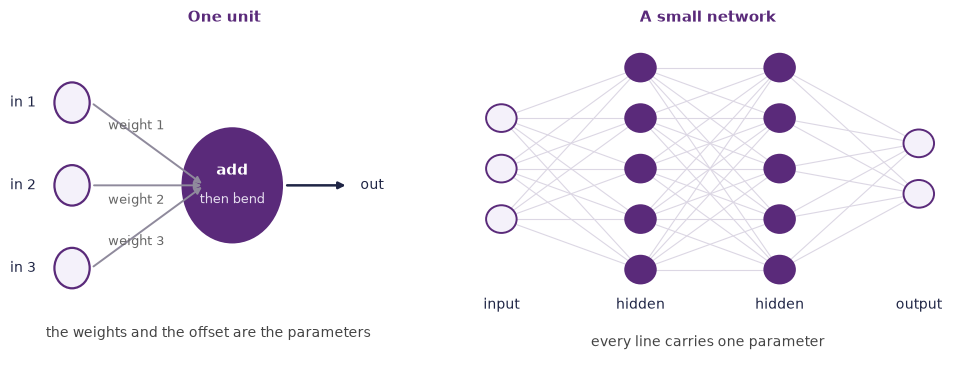
Figure: A unit multiplies each input by a weight, adds an offset and bends the result, and a network is many such units stacked in layers so that the bends compound.
The families you will hear named in the wild are mostly variations on that theme.
- Convolutional networks, which slide small parameter patches across an image, dominated computer vision for most of the 2010s.
- Recurrent networks, which pass a running summary from one time step to the next, were the standard for text and audio until around 2018 Karpathy, 2015.
- Transformers, introduced in 2017, let every element of a sequence look at every other element directly, and had become the dominant architecture by 2020 for language, and soon after for audio, image, and code Vaswani et al., 2017. That mechanism is called attention, and it is why a model can connect a word at the end of a paragraph to one at the beginning.
- Diffusion, which is a training and sampling procedure layered on top of a network rather than an architecture of its own, is treated in full in A taxonomy of generative models below, and applied in chapter 5.
The architecture matters a great deal for performance and cost. It does not change the cast of characters above, which is why you can follow the field without tracking every new acronym.
Dig deeper: what a layer computes
A single layer takes an input vector and computes .
is a matrix of parameters and a vector of parameters, so is a linear map: it can stretch, rotate, and shift the input, and nothing more. is a fixed non-linear function applied element by element, in practice usually a rectifier that sets negative values to zero.
The non-linearity is the whole trick. Without it, stacking a hundred layers would still only give you a linear map, because a composition of linear maps is linear. With it, each layer can bend the space a little, and a deep stack can carve out regions of astonishing complexity.
Training adjusts every entry of every and by gradient descent. A model with a trillion parameters is that same operation, repeated.
From classifying to generating
For most of its history, machine learning was used to classify: is this email spam, is this image a cat, does this scan show a tumour? Generative AI turns the question around. Instead of labelling an existing thing, the model produces a new one.
Suppose you have a dataset of pictures of cats. A classifier learns a function that says “given an image, output 1 if it is a cat and 0 otherwise”. A generator learns a different function: “produce an image that looks like the cats you have seen”.
The classifier learns a boundary, the line between cat and not-cat. The generator learns a distribution, the whole space of plausible cat pictures. The distribution is much harder to learn, because a boundary only has to be right near the line while a distribution has to be right everywhere. But once you have it, you can draw from it and get pictures that never existed.
Source
import numpy as np
from scipy.stats import gaussian_kde

import matplotlib.pyplot as plt
plt.rcParams.update({
    "font.size": 10,
    "axes.titlesize": 11,
    "axes.labelsize": 10,
    "xtick.labelsize": 9,
    "ytick.labelsize": 9,
    "legend.fontsize": 9,
    "figure.figsize": (10, 4),
    "figure.dpi": 100,
    "savefig.dpi": 150,
    "axes.spines.top": False,
    "axes.spines.right": False,
})

navy, purple, rose = "#1f2545", "#5a2a7a", "#e8556d"
rng = np.random.default_rng(7)

cats = np.vstack([rng.normal((3.2, 6.4), (0.9, 0.8), size=(70, 2)),
                  rng.normal((5.0, 4.4), (0.8, 0.7), size=(60, 2))])
others = rng.normal((7.2, 3.0), (1.2, 1.1), size=(110, 2))

fig, (left, right) = plt.subplots(1, 2, figsize=(10, 4.2), sharex=True, sharey=True)

left.plot(others[:, 0], others[:, 1], "o", color="#b9b4c4", markersize=4.5,
          label="not a cat")
left.plot(cats[:, 0], cats[:, 1], "o", color=purple, markersize=4.5, label="a cat")
xs = np.linspace(0.5, 9.5, 50)
left.plot(xs, 10.4 - 1.05 * xs, color=rose, lw=2.4, label="the boundary")
left.set_title("A classifier learns a boundary",
               fontweight="bold", color=purple)
left.legend(loc="lower left", frameon=False)

grid_x, grid_y = np.mgrid[0.5:9.5:80j, 0.5:9.5:80j]
density = gaussian_kde(cats.T)(np.vstack([grid_x.ravel(), grid_y.ravel()]))
right.contourf(grid_x, grid_y, density.reshape(grid_x.shape), levels=9, cmap="Purples")
right.plot(cats[:, 0], cats[:, 1], "o", color=purple, markersize=3, alpha=0.45)
sample = np.array([4.1, 5.4])
right.plot(*sample, "*", color=rose, markersize=20, zorder=5,
           markeredgecolor="white", markeredgewidth=1.2)
right.annotate("a new cat, drawn\nfrom the distribution", xy=sample,
               xytext=(6.4, 7.9), fontsize=10, color=rose, ha="center",
               arrowprops=dict(arrowstyle="-|>", color=rose, lw=1.4))
right.set_title("A generator learns a distribution",
                fontweight="bold", color=purple)

for ax in (left, right):
    ax.set_xlim(0.5, 9.5)
    ax.set_ylim(0.5, 9.5)
    ax.set_xticks([])
    ax.set_yticks([])
    ax.set_xlabel("two made-up features of an image", color="#444444")
    for side in ("right", "top"):
        ax.spines[side].set_visible(False)

plt.tight_layout()
plt.show()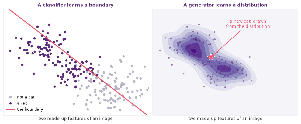
Figure: On the same made-up data a classifier draws the line between cat and not cat, while a generator learns the whole region the cats occupy and can draw a new point from it.
That sentence is the single mental shift behind everything else in this book, and it is what moved machine learning out of the back office and into the foreground of daily work after 2020.
Probability without tears
You do not need formal probability for this course, but two ideas will repay the five minutes.
Distributions
A distribution is a way of saying how likely each possible thing is. The heights of students at UiO form a distribution in which 1.70 m is common and 2.20 m is not. A generative image model implicitly learns a distribution over images, and a generative language model learns one over sequences of words.
The catch is scale. A single colour image is 786 432 numbers, so the space of all such images is unimaginably large, and almost all of it is noise. The set of plausible images is a vanishingly thin sliver inside that space. Learning to find and move around on that sliver is what diffusion models, adversarial networks, and transformers all do, by different routes.
This is also why the metaphor of a “database of stolen images” is technically wrong and rhetorically understandable. The model does not hold copies. It holds a compressed description of where the plausible region is, learned from copies it was shown. Whether that distinction should matter legally is a separate question, taken up in chapter 3, which also asks what kind of memory a compressed space like this one is and answers that it is not an archive.
Sampling
To sample is to draw one concrete thing from a distribution. Every time you press “generate”, the model is sampling. Press it twice and you get two different results, usually similar in character and never identical.
Samplers have knobs, and the knobs are where a lot of your aesthetic control lives.
- Temperature, in text and audio models, flattens or sharpens the distribution before the draw. High temperature makes the output more varied and stranger; low temperature makes it safer and more predictable, and at zero it stops being random at all.
- Top-k and top-p, in text models, restrict the draw to the most likely candidates, either the best k of them or the smallest set whose probabilities sum to p. This is what stops a model from occasionally sampling nonsense from the far tail.
- Guidance scale, in image and video models, strengthens the pull of your prompt against the model’s own sense of what is plausible. Too high and results turn rigid and oversaturated; too low and the prompt is politely ignored.
- Steps, in diffusion models, set how many denoising passes to take. More steps usually mean a cleaner result, with sharply diminishing returns.
Source
import numpy as np

import matplotlib.pyplot as plt
plt.rcParams.update({
    "font.size": 10,
    "axes.titlesize": 11,
    "axes.labelsize": 10,
    "xtick.labelsize": 9,
    "ytick.labelsize": 9,
    "legend.fontsize": 9,
    "figure.figsize": (10, 4),
    "figure.dpi": 100,
    "savefig.dpi": 150,
    "axes.spines.top": False,
    "axes.spines.right": False,
})

navy, purple, rose = "#1f2545", "#5a2a7a", "#e8556d"
tokens = ["quiet", "cold", "bright", "distant", "purple"]
scores = np.array([3.0, 2.2, 1.6, 0.9, -0.4])
temperatures = [0.3, 1.0, 1.8]

fig, axes = plt.subplots(1, 3, figsize=(10, 3.6), sharey=True)
for ax, temperature in zip(axes, temperatures):
    weights = np.exp(scores / temperature)
    probabilities = weights / weights.sum()
    colours = [rose] + [purple] * (len(tokens) - 1)
    ax.bar(tokens, probabilities, color=colours, width=0.62)
    for index, value in enumerate(probabilities):
        ax.text(index, value + 0.02, f"{value:.2f}", ha="center",
                fontsize=9, color="#444444")
    ax.set_title(f"temperature {temperature}",
                 fontweight="bold", color=purple)
    ax.tick_params(axis="x", labelrotation=35)
    for label in ax.get_xticklabels():
        label.set_horizontalalignment("right")
    for side in ("right", "top"):
        ax.spines[side].set_visible(False)

axes[0].set_ylim(0, 1.08)
axes[0].set_ylabel("probability of being drawn")
axes[1].set_xlabel("candidates for the word after \"the night was\"",
                   color="#444444", labelpad=8)
plt.tight_layout()
plt.show()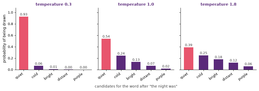
Figure: The same five scores become three different distributions as the temperature changes, so a low temperature concentrates the draw on the leading candidate and a high one spreads it out.
The same prompt with different sampler settings can produce dramatically different work. Internalising that is one of the most useful things you can do this semester, because it moves your attention from writing the perfect prompt to running a deliberate experiment.
Models, tools and versions
Two words are used almost interchangeably in everyday talk about AI, and keeping them apart settles a surprising number of arguments.
A model is the trained artefact described earlier in this chapter: the network plus one specific set of parameter values, frozen in a file. Models are published under a family name, a version, and often a size. One family may ship as a small, a medium, and a large variant, and each of them is retrained and renumbered every few months. A model does one thing. It maps an input to an output, and it has no interface, no memory of you, and no terms of service.
A tool is a product built around one or more models. Around the model sit an interface, a system prompt you never see, sometimes retrieval from documents or the web, sometimes a stored memory, plug-ins or tool calls, safety filters, a data policy, and a price. Every one of those parts changes what comes back. It is the tool, and not the model, that decides what happens to the words you type. The tool decides what is added to them, what is searched, what is refused, and what is logged.
The relation between the two runs in both directions. One model turns up inside a chat app, an assistant living in a code editor, and an image app in the browser, and behaves differently in each because each wraps it differently. A single tool can also switch models between two sessions without saying so, or change the system prompt behind a name that stays the same. An output that was good last week and is odd today is therefore as likely to be a tool change as a model change.
Three practical consequences follow, and they run through the rest of the course. Record both the tool and the model, with its version or the date, in your practice log and in every declaration of AI use. The tool is what a reader can reproduce, and the model is what your claim is about. Compare two models by holding the tool constant, and two tools by holding the model constant, or the comparison measures nothing. Read the tool’s data policy, since the model does not have one.
In the vocabulary of the five layers, the model sits at the model layer and the tool at the interface layer. Naming which of the two you mean is the first move in most of the questions this book asks.
Steering the model
Conditioning
If a generator simply samples from its full distribution, you get something randomly cat-shaped, which is useful as a demonstration and useless as work. The technical word for steering the generator is conditioning.
Conditioning is anything fed to the model in addition to noise in order to bias what comes out.
- A text prompt is the most common form.
- A reference image conditions on appearance: make it look like this.
- A mask conditions on location: change only this part.
- A control signal such as a pose skeleton, an edge map, or a depth map conditions shape and composition, and is the basis of the structural control tools discussed in chapter 5.
- An audio waveform or a symbolic score conditions a music model, as chapter 6 explores.
- A previous frame conditions the next one in a video model, which is chapter 7.
Source
from matplotlib.patches import FancyBboxPatch

import matplotlib.pyplot as plt
plt.rcParams.update({
    "font.size": 10,
    "axes.titlesize": 11,
    "axes.labelsize": 10,
    "xtick.labelsize": 9,
    "ytick.labelsize": 9,
    "legend.fontsize": 9,
    "figure.figsize": (10, 4),
    "figure.dpi": 100,
    "savefig.dpi": 150,
    "axes.spines.top": False,
    "axes.spines.right": False,
})

navy, purple, rose = "#1f2545", "#5a2a7a", "#e8556d"
inputs = ["Text prompt", "Reference image", "Mask", "Control signal"]

fig, ax = plt.subplots(figsize=(10, 4.4))
for i, name in enumerate(inputs):
    y = 4.4 - i * 1.2
    ax.add_patch(FancyBboxPatch((0.4, y), 2.8, 0.9,
                                boxstyle="round,pad=0.02,rounding_size=0.12",
                                facecolor="#f4f1fa", edgecolor=purple, linewidth=1.8))
    ax.text(1.8, y + 0.45, name, ha="center", va="center", fontsize=11, color=navy)
    ax.annotate("", xy=(4.9, 3.4 - i * 0.28), xytext=(3.3, y + 0.45),
                arrowprops=dict(arrowstyle="-|>", color=navy, lw=1.8))

ax.add_patch(FancyBboxPatch((5.0, 2.3), 2.6, 1.4,
                            boxstyle="round,pad=0.02,rounding_size=0.18",
                            facecolor=purple, edgecolor=purple, linewidth=2))
ax.text(6.3, 3.0, "Generative\nmodel", ha="center", va="center",
        fontsize=11, fontweight="bold", color="white")

ax.add_patch(FancyBboxPatch((8.8, 2.3), 2.6, 1.4,
                            boxstyle="round,pad=0.02,rounding_size=0.15",
                            facecolor="#fff0f3", edgecolor=rose, linewidth=1.8))
ax.text(10.1, 3.0, "Image, sound,\nvideo, text", ha="center", va="center",
        fontsize=11, color=navy)
ax.annotate("", xy=(8.8, 3.0), xytext=(7.6, 3.0),
            arrowprops=dict(arrowstyle="-|>", color=navy, lw=1.8))

ax.set_xlim(0, 11.8)
ax.set_ylim(0.4, 5.6)
ax.axis("off")
plt.tight_layout()
plt.show()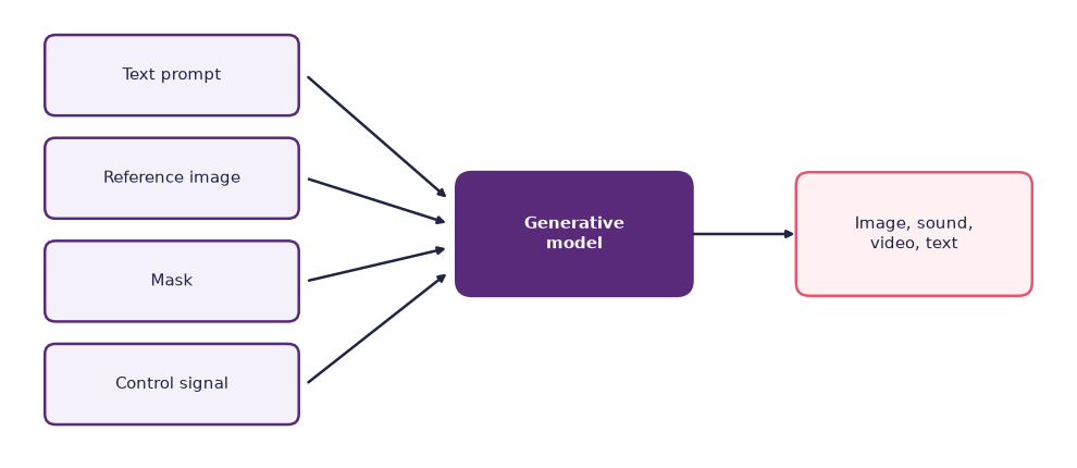
Figure: A text prompt, a reference image, a mask, and a control signal are four ways to condition one generative model. The model is shared; the inputs change.
Once you start looking for it, you see conditioning everywhere. The user interface of every generative tool is essentially a conditioning console, and the difference between a toy and a professional tool is mostly how many conditioning channels it exposes and how precisely.
Prompts as the new interface
For a generation of users who have never seen a command line, prompts are the new interface. A prompt is just text, but writing a good one has become its own small craft, and the tips and tricks page collects the moves that transfer between tools. Five principles hold nearly everywhere.
- Be specific about subject, style, context, and constraint. Vagueness is answered with the average of the training data.
- Show rather than only tell. Quote a sentence, paste an example, attach an image. One example is worth a paragraph of adjectives.
- Iterate. Generation is cheap, so treat the first output as a draft and the second as the first real attempt.
- Constrain the form, not only the content: in three sentences, as a bulleted list, as a poster in a 1:2 ratio.
- Inspect failures. When an output is wrong, write down how it is wrong. That description is usually a better next prompt than your first one was.
Chapter 4 takes prompting for language models seriously. For now the point is structural: the prompt is the interface, the interface is text, and text is a lossy encoding of what you actually want.
Three ways to make a machine generate
Everything so far has described one way of building a generative machine: show it examples and let it work out the pattern. That is the dominant way in 2026 and it is not the only one. Two older families are still in daily use by artists, composers, game developers, and roboticists, and holding all three in view makes it much easier to see what any given tool is actually doing.
Rule-based systems come first. You write the rules and the machine applies them. A grammar rewrites symbols into other symbols, so an L-system can grow a plant from four rewriting rules. A cellular automaton updates a grid from the states of each cell’s neighbours, as in Conway’s Game of Life. A Markov chain draws the next note from a table of transition probabilities, and a constraint solver fills a level layout without ever breaking a condition you stated. The tradition’s landmarks are systems that ran for years: AARON, which drew and later painted from Harold Cohen’s rules McCorduck, 1991, and David Cope’s Experiments in Musical Intelligence, which recombined a composer’s own phrases under rules Cope wrote by hand Cope, 1991. What the maker specifies is the whole process.
Evolutionary computation comes second. Here you do not write the process, you write the score. Start with a population of candidates, vary them by mutation and crossover, keep the ones that score well, repeat. The score is the fitness function. When you cannot write one, you can be one: in interactive evolution a person picks favourites each round and the machine breeds from those. Dawkins’s biomorphs worked that way in 1986, and Picbreeder did the same in a browser two decades later Dawkins, 1986Secretan et al., 2008. Artists have evolved images and sculptural forms this way since the early 1990s Sims, 1991Todd & Latham, 1992, and Eiben and Smith is the standard textbook Eiben & Smith, 2015. What the maker specifies is a way of judging rather than a way of making.
Learned models come third, and they are the rest of this chapter. You supply the data and the objective, and the process is found by the training loop.
| Rule-based | Evolutionary | Learned | |
|---|---|---|---|
| What you specify | the rules themselves | a fitness function, or your own eye | a dataset and an objective |
| Where novelty comes from | simple rules interacting over many steps | random variation, kept when it scores well | sampling from a learned distribution |
| Good at | control, low cost, endless variation inside a style you set | searching spaces you cannot describe, and surprising you | breadth, realism, and following an instruction written in ordinary language |
| Weaknesses | anything you cannot state as a rule | slowness, and inheriting every flaw in your score | fine control, cost, and explaining why it produced what it did |
| Typical creative uses today | procedural generation in games, plant and terrain modelling, algorithmic composition | evolved shapes and sounds, interactive breeding of designs, evolved robot controllers | text, image, audio, and video generation |
The three are not rivals, and modern pipelines mix them freely. A studio lays out a level with rules and fills its surfaces with generated textures. An artist runs an evolutionary loop over prompts, or over points in a model’s latent space, the compressed set of numbers a trained model works in, using the learned model as the thing being searched. A search procedure calls a learned model to score its own candidates. When a pipeline is described simply as “AI”, it is worth asking which family is doing which part, because the answer tells you where the control sits and who put it there.
You meet the older two again as material rather than history. Chapter 9 puts rule-based generative art and interactive evolution into a browser sketch you write yourself, and chapter 12 meets robot behaviour that was evolved rather than designed or learned. And if you want to watch the second family run, the evolutionary loop in the Dig deeper notes at the end of this chapter fits the same two-parameter line as the training loop, without a single gradient.
The model landscape
A taxonomy of generative models
Four families cover almost everything you will meet.
- Generative adversarial networks train two networks against each other, a generator producing samples and a discriminator trying to tell them from real data Goodfellow et al., 2014. They dominated image generation from 2014 to about 2020 and are now largely retired, having proved hard to train and hard to steer.
- Autoregressive models predict the next element given the previous ones, factorising a distribution over sequences into a chain of small predictions. This powers every chat model and a good deal of audio and image generation.
- Diffusion models learn to denoise. Starting from pure noise, the model removes a little at a time until a coherent image, sound, or video emerges Ho et al., 2020. Doing the denoising in a compressed latent space rather than on raw pixels is what made high-resolution generation practical on ordinary hardware Rombach et al., 2022.
- Flow matching, a close cousin of diffusion with a simpler training objective, powers several of the strongest image and video models released from 2024 onwards Esser et al., 2024.
You do not need to memorise this. But when a tool advertises itself as adversarial, autoregressive, diffusion-based, or flow-based, you should be able to nod and know roughly what follows for speed, controllability, and failure modes.
Foundation models and fine-tuning
Most creative AI tools in 2026 are built on foundation models: very large models trained once at enormous cost, then adapted to many tasks by people who could never afford to train one. Adaptation takes four common forms.
- Prompting puts the right text in front of a frozen model at inference time. Nothing is retrained, and the effect lasts only as long as the conversation.
- Fine-tuning continues training a foundation model briefly on a smaller, focused dataset. Costs range from a few euros for a lightweight adapter on a rented GPU to millions for a full fine-tune of a large model.
- Alignment training, using human or model-generated feedback, shapes a raw next-token predictor into something that answers questions, follows instructions, and refuses some requests.
- Distillation trains a smaller student model to imitate a larger teacher, which is how capable models end up running on a phone.
This layering has an economic consequence worth naming early. A handful of organisations can afford to build foundation models, and everybody else builds on top. That concentration shapes what tools exist, what they cost, and what they will not let you do, which is a culture-layer question that chapter 3 returns to.
For most of this course you will be prompting existing foundation models rather than training anything.
What generative models cannot do
A short list, worth keeping beside you all semester.
- They do not know what is true. A text model can produce a fluent paragraph that is factually wrong, and an image model can produce a hand with six fingers, for the same reason: both are sampling what is plausible, and plausibility is not truth.
- They generalise from data, not from causal understanding. There is no model of physics inside, no model of social cause, no account of why anything happens. Patterns that held in the data are extended; patterns that did not are not discovered.
- They are not deterministic at default settings. Same prompt, different output, which is a feature when you are exploring and a problem when you need a result you can reproduce. Fix the seed and the sampler settings if reproducibility matters.
- They do not remember you between sessions unless they were explicitly built to, with retrieval, stored notes, or fine-tuning. What looks like memory is usually text quietly pasted back into the input.
- They are bounded by a training cutoff. Anything more recent is invisible unless the system can search or read files you provide.
Every one of these limits is a design constraint rather than a temporary bug. Working well with these systems is therefore less like using a tool and more like managing a collaborator with a strange and specific set of blind spots. Chapter 3 turns that observation into a working practice, through five paradoxes of co-creation and the shift from craftsperson to creative director.
Three more optional deep dives follow, two on the loops that fit a model and one on sampling. You can skip all three and still pass the course.
Dig deeper: a 12-line training loop
The figure below is the whole of machine learning at the smallest possible scale. Behind it lie 200 noisy points that sit roughly on a line, and a model with exactly two parameters, a slope and an offset, fitted to them by running the four-step loop from the Training section 200 times.
Expand the code and read it against the pipeline figure at the top of the chapter. There, pred is the prediction and loss is the loss; the two grad lines say which direction each parameter should move, and the last two lines take the step. Everything you will use this semester is this loop scaled up by a factor of ten billion. It runs when the book is built, so the numbers and the figure below are real output, not a screenshot.
Source
import numpy as np

import matplotlib.pyplot as plt
plt.rcParams.update({
    "font.size": 10,
    "axes.titlesize": 11,
    "axes.labelsize": 10,
    "xtick.labelsize": 9,
    "ytick.labelsize": 9,
    "legend.fontsize": 9,
    "figure.figsize": (10, 4),
    "figure.dpi": 100,
    "savefig.dpi": 150,
    "axes.spines.top": False,
    "axes.spines.right": False,
})

rng = np.random.default_rng(0)
x = rng.uniform(-1, 1, size=200)
y = 2 * x + 0.5 + rng.normal(0, 0.1, size=200)

w, b, lr = 0.0, 0.0, 0.05

for step in range(200):
    pred = w * x + b
    loss = ((pred - y) ** 2).mean()
    grad_w = ((pred - y) * x).mean() * 2
    grad_b = (pred - y).mean() * 2
    w -= lr * grad_w
    b -= lr * grad_b

print(f"w = {w:.3f}, b = {b:.3f}, loss = {loss:.4f}")

grid = np.linspace(-1, 1, 100)
plt.scatter(x, y, s=8, alpha=0.4, label="training examples")
plt.plot(grid, w * grid + b, color="crimson", label="fitted model")
plt.xlabel("x")
plt.ylabel("y")
plt.title("A two-parameter model fitted by gradient descent")
plt.legend()
plt.tight_layout()
plt.show()
w = 1.986, b = 0.492, loss = 0.0104
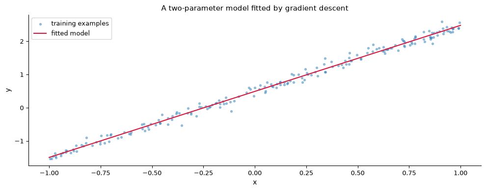
The recovered parameters land near the 2 and the 0.5 the data was built from, and the red line sits through the middle of the cloud. Nothing in the loop was told what a line is. It only ever knew whether the last guess was too high or too low.
Dig deeper: an evolutionary loop in twelve lines
The figure below fits the same two-parameter line as the figure above, on the data built the same way, and it does so without computing a single gradient. It keeps 50 candidate (w, b) pairs, scores each by how badly it fits, discards the worst 40, and refills the population by copying the survivors with a little random noise added. Sixty rounds of that is enough.
Read the curve beside the gradient-descent figure above and notice what is absent. Nothing here knows which direction is downhill. The population finds out by trying, which is why the curve falls in ragged steps rather than smoothly.
Source
import numpy as np

import matplotlib.pyplot as plt
plt.rcParams.update({
    "font.size": 10,
    "axes.titlesize": 11,
    "axes.labelsize": 10,
    "xtick.labelsize": 9,
    "ytick.labelsize": 9,
    "legend.fontsize": 9,
    "figure.figsize": (10, 4),
    "figure.dpi": 100,
    "savefig.dpi": 150,
    "axes.spines.top": False,
    "axes.spines.right": False,
})

rng = np.random.default_rng(0)
x = rng.uniform(-1, 1, size=200)
y = 2 * x + 0.5 + rng.normal(0, 0.1, size=200)

pop = rng.normal(0, 1, size=(50, 2))
history = []

for gen in range(60):
    pred = pop[:, :1] * x + pop[:, 1:]
    loss = ((pred - y) ** 2).mean(axis=1)
    order = np.argsort(loss)
    parents = pop[order[:10]]
    history.append(loss[order[0]])
    children = parents[rng.integers(0, 10, size=40)] + rng.normal(0, 0.1, size=(40, 2))
    pop = np.vstack([parents, children])

w, b = pop[0]
print(f"w = {w:.3f}, b = {b:.3f}, loss = {history[-1]:.4f}")

plt.plot(history)
plt.xlabel("generation")
plt.ylabel("best loss in the population")
plt.title("The same line fitted by evolution instead of gradients")
plt.tight_layout()
plt.show()
w = 1.988, b = 0.490, loss = 0.0104
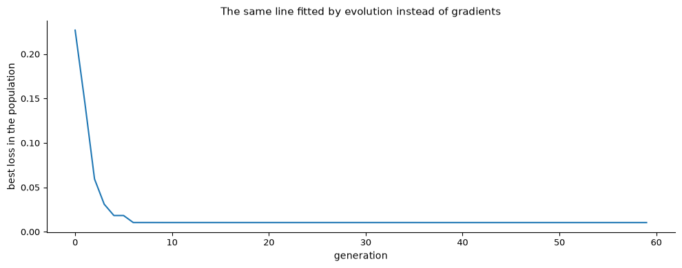
The evolutionary run lands close to the same slope and offset as the gradient-descent run above, by a completely different mechanism. The difference that matters is what each loop needs in order to run at all. The gradient loop needs the loss to be differentiable, so that a direction can be computed, while the evolutionary loop needs only that you can score a candidate. That is why evolution survives in places gradients cannot go.
Dig deeper: sampling from a tiny language model
The listing below shows the temperature knob directly. It loads GPT-2, a small and by 2026 rather quaint language model, and generates from the same opening at three temperatures. Low temperature gives you the safe continuation every time; high temperature wanders, sometimes usefully. This one is not run when the book is built, because it downloads several hundred megabytes of model weights, but it will run on a laptop.
from transformers import pipeline

gen = pipeline("text-generation", model="gpt2")

for t in [0.2, 0.7, 1.2]:
    out = gen("Once upon a time in Oslo,", max_new_tokens=40, temperature=t, do_sample=True)
    print(f"--- t={t} ---")
print(out[0]["generated_text"])This week’s lab: Explore, Reflect, Create
This lab makes the two halves of the chapter concrete: where a model comes from, and what happens when you turn its knobs.
Explore (about 30 min)
- Read one model card. Go to Hugging Face, search for an image or text model that interests you, and open its model card. Find four things and write them in your log: which dataset it was trained on, how many parameters it has, what licence it carries, and what limitations the authors admit to. Note anything you cannot find, because the gaps are as informative as the answers.
- Same prompt, three samplers. In an image tool, write one prompt with a clear subject and style, for example a watercolour illustration of a fox reading in a library, warm tones, soft light. Generate it three times: at the default setting, at a distinctly lower guidance or temperature, and at a distinctly higher one. Change nothing else. Save all three with their settings. Use a tool that exposes guidance or temperature as a number you can type, because a service that hides its settings will not let you attribute the difference to anything.
- Optional. Run the training loop playground and the next-token sampler if you would rather see the loop and the knob than read about them.
Reflect (about 15 min)
Work in pairs, then in plenary. This is a discussion, not a writing block.
- Explain to your partner, without notes, the difference between learning a boundary and learning a distribution, and say why the difference matters for the kind of work you want to make.
- Put your three samples side by side. What exactly changed between them, and which of the three would you defend to a client? Compare that answer with the sentence you wrote at the start of the chapter about what happens when you press “generate”.
- Close the round by stating one intention aloud: one thing you now intend to make in the next 45 minutes, and which knob you will use to get there.
Create (about 45 min)
- Compose a triptych from your three samples: three panels side by side, each captioned with the one parameter that produced it. Aim for something that reads as a piece of work rather than a screenshot grid.
- Write a 150-word artist’s statement to sit under it, framing the triptych as an experiment you designed. Say what you were testing, what surprised you, and which panel you would keep.
- Swap with another pair in the last 15 minutes and try to guess each other’s settings from the panels alone.
At home, write this week’s entry in your practice log using the practice log template. Carry the triptych into your portfolio.
A1, the AI-augmented self-introduction, is due this week; the overview sets out what to hand in. Keep the feedback you receive on it, since a revised A1 goes into your portfolio.
A critical look: is a language model just autocomplete?
The claim. A large language model is “just autocomplete”: a statistical next-word predictor with no understanding, and any appearance of reasoning is an illusion produced by scale.
The evidence. The first half of the claim is simply true, and the model builders say so. The training objective of a base language model is to predict the next token in a sequence, which is precisely what a phone keyboard does with a much smaller model. What complicates the picture is what fell out of doing that at scale. Models trained this way turned out to perform tasks they were never trained on when shown a few examples in the prompt, a behaviour reported at scale in 2020 Brown et al., 2020. A widely cited 2022 survey then catalogued abilities that appeared to be absent in smaller models and present in larger ones, calling them emergent Wei et al., 2022.
The method. That second finding is where care is needed. Emergence was measured on benchmarks, and many benchmarks score answers as exactly right or exactly wrong. Under a metric like that, a model whose internal accuracy is improving smoothly will look flat until it crosses the threshold, then appear to jump. Later work re-scored some of the same results with continuous metrics and watched the jumps flatten into curves Schaeffer et al., 2023. The abilities were real; the sharp discontinuity was partly an artefact of how they were counted. Neither result was designed to test whether the model understands anything, because no benchmark of this kind can.
The limits. Both slogans over-claim. “Just autocomplete” describes the training objective and then quietly infers a conclusion about capability, which does not follow: evolution is just differential reproduction, and that tells you little about what an eye can do. “It understands” imports a word from human psychology that nothing in the evidence licenses. The question that actually pays rent is narrower and answerable: what can this model do reliably on my task, and how would I know? You can settle that in an afternoon with twenty test cases of your own, and you should, for any task you plan to trust it with.
- Strubell, E., Ganesh, A., & McCallum, A. (2019). Energy and Policy Considerations for Deep Learning in NLP. Proceedings of the 57th Annual Meeting of the Association for Computational Linguistics (ACL), 3645–3650. 10.18653/v1/P19-1355
- Bender, E. M., Gebru, T., McMillan-Major, A., & Shmitchell, S. (2021). On the Dangers of Stochastic Parrots: Can Language Models Be Too Big? Proceedings of the ACM Conference on Fairness, Accountability, and Transparency (FAccT). 10.1145/3442188.3445922
- Crawford, K. (2021). Atlas of AI: Power, Politics, and the Planetary Costs of Artificial Intelligence. Yale University Press. https://yalebooks.yale.edu/book/9780300264630/atlas-of-ai/
- Goodfellow, I., Bengio, Y., & Courville, A. (2016). Deep Learning. MIT Press. https://www.deeplearningbook.org/
- Karpathy, A. (2015). The Unreasonable Effectiveness of Recurrent Neural Networks. https://karpathy.github.io/2015/05/21/rnn-effectiveness/
- Vaswani, A., Shazeer, N., Parmar, N., Uszkoreit, J., Jones, L., Gomez, A. N., Kaiser, L., & Polosukhin, I. (2017). Attention Is All You Need. Advances in Neural Information Processing Systems (NeurIPS). https://arxiv.org/abs/1706.03762
- McCorduck, P. (1991). AARON’s Code: Meta-Art, Artificial Intelligence, and the Work of Harold Cohen. W.\,H. Freeman. https://archive.org/details/aaronscodemetaar0000mcco
- Cope, D. (1991). Computers and Musical Style. A-R Editions. https://www.worldcat.org/isbn/0895792567
- Dawkins, R. (1986). The Blind Watchmaker. Longman. https://www.worldcat.org/isbn/0582446945
- Secretan, J., Beato, N., D’Ambrosio, D. B., Rodriguez, A., Campbell, A., & Stanley, K. O. (2008). Picbreeder: Evolving pictures collaboratively online. Proceedings of the SIGCHI Conference on Human Factors in Computing Systems. 10.1145/1357054.1357328
- Sims, K. (1991). Artificial evolution for computer graphics. ACM SIGGRAPH Computer Graphics, 25(4), 319–328. 10.1145/127719.122752
- Todd, S., & Latham, W. (1992). Evolutionary Art and Computers. Academic Press. https://www.worldcat.org/isbn/0124371851
- Eiben, A. E., & Smith, J. E. (2015). Introduction to Evolutionary Computing (2nd ed.). Springer. 10.1007/978-3-662-44874-8
- Goodfellow, I. J., Pouget-Abadie, J., Mirza, M., Xu, B., Warde-Farley, D., Ozair, S., Courville, A., & Bengio, Y. (2014). Generative Adversarial Nets. Advances in Neural Information Processing Systems (NeurIPS). https://arxiv.org/abs/1406.2661
- Ho, J., Jain, A., & Abbeel, P. (2020). Denoising Diffusion Probabilistic Models. Advances in Neural Information Processing Systems (NeurIPS). https://arxiv.org/abs/2006.11239