Video Analysis

All video analysis methods are called on an MgVideo object. Each method writes output files alongside the source video and returns a result object you can use directly or pass to further methods.

import musicalgestures as mg

mv = mg.MgVideo('/path/to/video.avi')

Which method should I use?

Several methods have overlapping or similar-sounding names. This table disambiguates the most commonly confused pairs — one line each:

Method	Use it when you want…
average()	a long-exposure mean of all frames — it is a convenience alias for blend(component_mode='average').
blend()	to composite all frames with a chosen mode ('average', 'lighten', 'darken', …).
history()	a video where each frame carries a trail of overlaid past frames.
motionhistory()	a single Motion History Image — one image where brightness encodes when motion last happened (recency).
motion().average() / heatmap()	a single motion-density image — where and how much motion happened (order-independent).
motiongrams()	how motion (frame differences) is distributed in space over time.
videograms()	how the raw pixel intensity (the whole scene, not motion) is distributed in space over time.
ssm() on MgVideo	self-similarity from visual features (features='motiongrams'/'videograms').
ssm() on MgAudio	self-similarity from audio features (features='spectrogram'/'chromagram'/'tempogram').
pose_waterfall()	pose markers flowing through (x, time, y) space (needs pose data).
silhouette_waterfall()	the silhouette profile cascading over a time axis (no pose needed).
motiontempo()	the dominant movement tempo (from the quantity-of-motion signal).
motiondescriptors()	scalar summaries of how something moves: motion energy, smoothness (SPARC), entropy, and spectral descriptors.
audio tempo() / tempogram()	the audio tempo / rhythmic periodicity.
tempo_similarity()	to compare movement tempo against audio tempo.

AVI conversion (convert)

Most analysis methods stream frames straight through FFmpeg and run on any container, including MP4 — e.g. motion(), motiongrams(), average()/blend(), videograms(), heatmap(), eulerian(), motiontempo(), sonomotiongram(), grid(), subtract(), and history().

A few methods that decode frame-by-frame with OpenCV first convert the input to an all-intra MJPEG .avi (cached once as self.as_avi) for frame-accurate decoding: flow.dense()/flow.sparse(), directograms(), impacts(), motion_mp(), and history_cv2(). The motion video output is also written as .avi.

If your MP4 decodes reliably and you want to skip that conversion (faster, no extra file), pass convert=False:

mv = mg.MgVideo('clip.mp4')
mv.flow.dense(convert=False)
mv.directograms(convert=False)

For these methods the default convert=True keeps the safe, frame-accurate behaviour.

pose() is different: its convert defaults to None ("auto"). The MediaPipe backend (the default) reads the source file directly, with no intermediate AVI; the OpenPose backends still convert for frame-accurate decoding. The pose result video is written in the original container — an mp4 in gives an mp4 out, with no avi→mp4 round-trip. Pass convert=True/False to force conversion on or off regardless of backend.

---

Threshold and filter parameters

Many methods accept threshold and filtertype:

• threshold (float, 0–1): pixels with a value below this fraction of 255 are set to zero. The default is 0.05. Higher values remove more background noise but may lose subtle motion.
• filtertype (str): 'Regular' (default) thresholds and median-filters; 'Binary' binarises the output; 'Blob' applies erosion instead.

See the filter reference for details.

---

Motion analysis

motion() is the primary analysis method. It renders a motion video, horizontal and vertical motiongrams, a motion plot, and a CSV of per-frame motion data, all in one call. It returns an MgVideo pointing to the motion video.

motion_video = mv.motion()      # returns MgVideo
motion_video.show()
mv.show(key='motion')           # equivalent shorthand

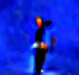
The motion video: bright where the image changes between frames.

Shortcuts

motion_vid = mv.motionvideo()   # motion video only — returns MgVideo

motiondata = mv.motiondata()    # CSV only — returns list of paths
motiondata = mv.motiondata(motion_analysis='aom')

motionplots = mv.motionplots()  # motion plot image — returns MgImage
motionplots = mv.motionplots(audio_descriptors=True)
motionplots.show()
mv.show(key='plot')

motiongrams = mv.motiongrams()        # returns MgList[MgImage, MgImage]
motiongrams[0].show()                 # horizontal motiongram
motiongrams[1].show()                 # vertical motiongram
motiongrams.show(key='horizontal')    # select a panel by orientation
motiongrams.show(key='vertical')
mv.show(key='horizontal')             # shorthand from the source MgVideo
mv.show(key='vertical')

score = mv.motionscore()        # average VMAF motion score — returns float

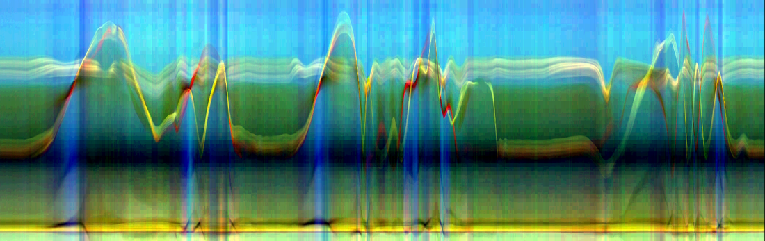
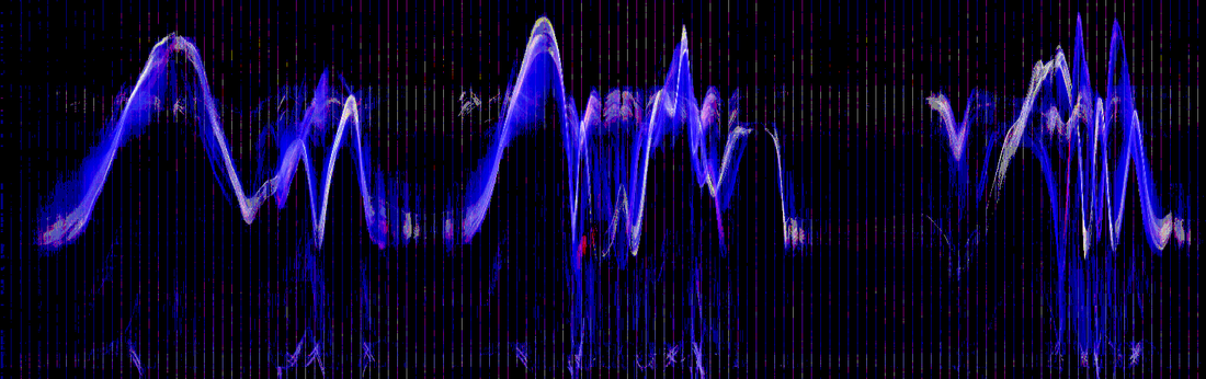Horizontal motiongram: vertical motion collapsed onto the y-axis, flowing left→right over time.

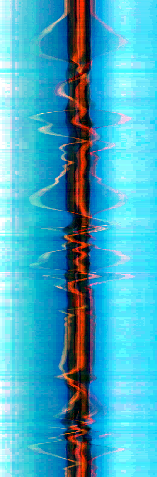
Vertical motiongram: horizontal motion collapsed onto the x-axis, stacked top→bottom over time.

Motion data columns

The CSV produced by motion() and motiondata() contains one row per frame:

Column	Description
Time	Frame timestamp in milliseconds
Qom	Quantity of motion (sum of active pixels)
ComX, ComY	Centroid of motion (normalised 0–1)
AomX1, AomY1, AomX2, AomY2	Bounding box of motion area (normalised)

---

Motion heatmap

heatmap() accumulates the absolute frame-to-frame difference across the whole video into a single colour-mapped image, so hot regions mark where the most change happened. By default the heat is overlaid on a dimmed average frame for spatial context.

heat = mv.heatmap()                                    # returns MgImage
heat = mv.heatmap(colormap='jet', overlay=False)       # bare heatmap on black
heat = mv.heatmap(blur=3, gamma=0.4, colormap='viridis')
heat.show()

Heatmap: accumulated frame-to-frame difference, hot colours mark where the most change happened, overlaid on the dimmed average frame.

• colormap: any matplotlib colormap ('inferno' default)
• overlay: composite on the dimmed average frame (default True); alpha/background_dim tune the mix
• blur: optional Gaussian smoothing radius; gamma (<1) boosts faint motion
• normalize: scale the most active pixel to the top of the colormap

---

Space-time visualisations

Several ways to show where a person is and when, in a single image. Silhouettes are extracted with MediaPipe selfie segmentation when available, else by background subtraction against the average frame (best for static-camera recordings). Control extraction with method='auto'|'mediapipe'|'bgsub'.

# Stroboscope / chronophotography — silhouettes at sampled times on one frame
mv.stroboscope(n_samples=12).show()

# 3D silhouette waterfall — silhouette profile cascading along a time axis
mv.silhouette_waterfall(n_samples=40, axis='horizontal').show()
mv.silhouette_waterfall(axes=False).show()   # clean render, no axes/labels/title

# Motion History Image — intensity = how recently motion happened (no silhouette needed)
mv.motionhistory().show()

# 3D space-time silhouette volume — (x, y, t) point cloud
mv.spacetime_volume(n_samples=50).show()

Stroboscope: silhouettes sampled at several times and composited onto a single frame (chronophotography).

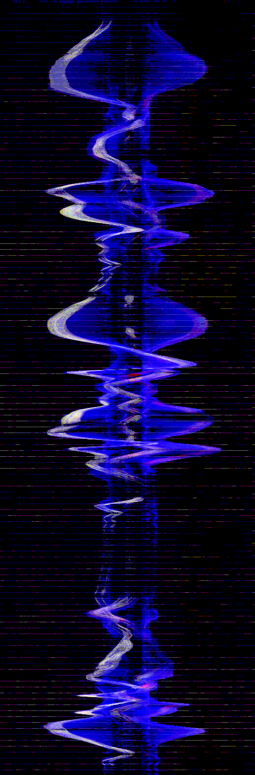
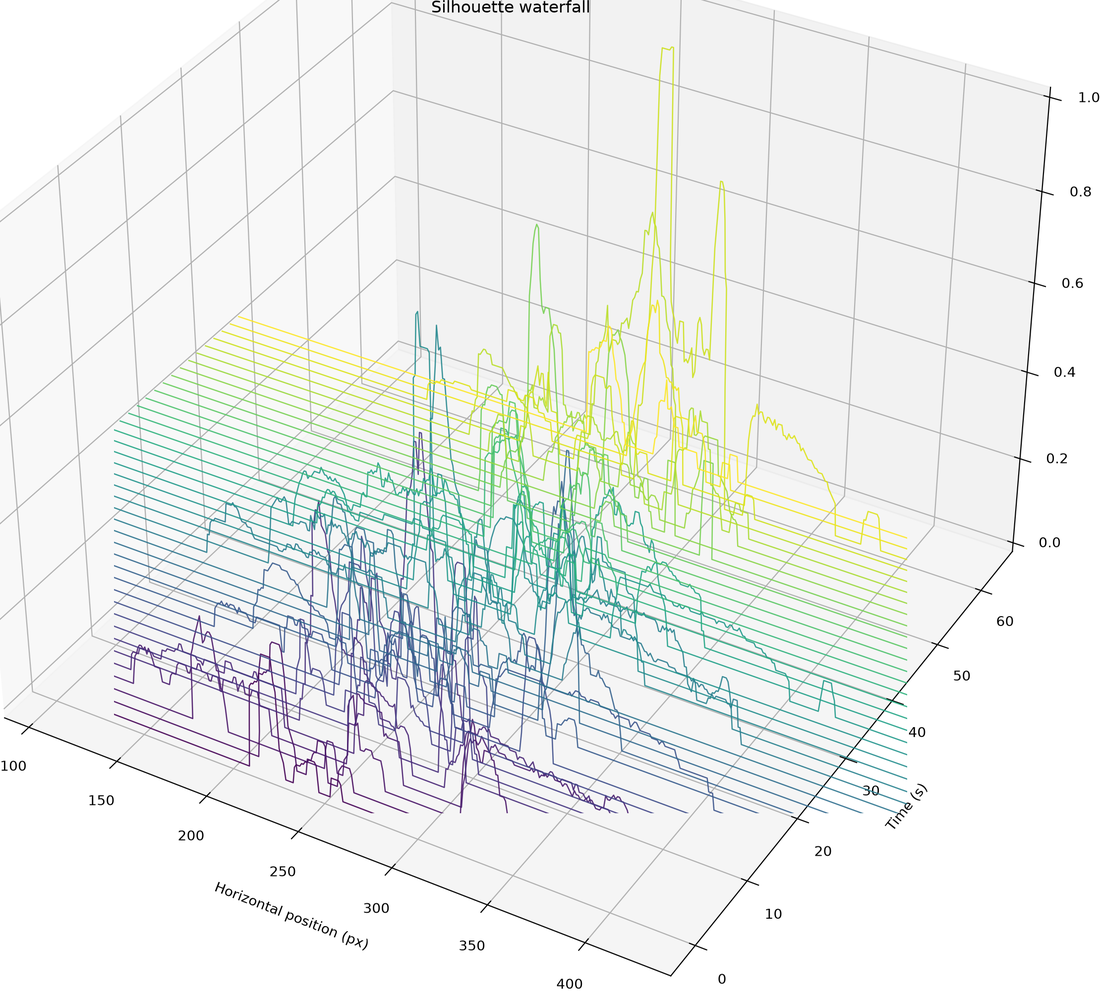Silhouette waterfall: the silhouette profile cascading along a time axis in 3D.

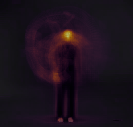
Motion History Image: brightness encodes how recently motion happened at each pixel (recent = bright, old = fades).

Cleaner silhouettes (single person on a static background). The silhouette methods (stroboscope, silhouette_waterfall, spacetime_volume) share controls: raise threshold to reject background noise, tune the morphological kernel_size, and set keep_largest=True to keep only the person's blob. If a result looks washed out / "blows up", these are the knobs:

mv.stroboscope(n_samples=10, threshold=0.15, keep_largest=True).show()

Motion History Image controls. motionhistory() decays old motion over a window so it doesn't accumulate and blow out: decay (fraction of the clip a mark persists; smaller = shorter trails), threshold (motion sensitivity), blur (speckle suppression), and normalize. normalize now defaults to False — the MHI is already built in [0, 1], and normalising rarely helps; when the final frames are static it amplified faint residual trails and over-brightened the image. (It is also guarded to skip when peak intensity is very low.) Set normalize=True to opt in:

mv.motionhistory(threshold=0.08, decay=0.2, blur=1).show()

These complement the motiongram (space×time) and the combined motion SSM (temporal structure): the stroboscope and volume show the body moving through space over time, the waterfall shows spatial occupancy flowing over time, and the MHI compresses recency of motion into one frame.

Density vs. recency: motionhistory() vs heatmap() / motion().average()

These single-image summaries look similar but encode different things — the distinction is whether time order matters:

Visualisation	Each pixel encodes	Time order
heatmap() and motion().average()	how much / how often motion happened there (motion density)	Order-independent — reversing or shuffling the frames gives the same image
motionhistory() (MHI)	when motion last happened there (motion recency: recent = bright, old = fades)	Order-dependent — reversing the video inverts the image

Concrete example — a dancer crossing the frame left → right:

• heatmap() / motion().average() → a uniformly bright band along the whole path (you can't tell which way they went).
• motionhistory() → a gradient along the path: dark where they were early, bright where they were recently — so you can read the direction and progression of the movement.

In short: use heatmap() / motion().average() for where and how much motion (a long-exposure of motion intensity); use motionhistory() for where and when (a recency map that captures the arrow of time).

Related but different: motion().history() (or mv.show(key='motionhistory')) is a video where each frame carries a short motion trail of the last N frames (a weighted moving average), rather than a single whole-clip summary image.

Note: motion() applies your threshold/filtertype when defining motion, whereas motionhistory() uses its own simple internal frame-difference threshold — so what counts as "motion" can differ slightly.

---

Movement tempo

motiontempo() estimates the dominant movement tempo from the quantity of motion (mean absolute frame difference) via an FFT, reported in both Hz and BPM.

mt = mv.motiontempo()                       # returns MgFigure
print(mt.data['tempo_bpm'])                 # dominant tempo in BPM
print(mt.data['dominant_frequency'])        # in Hz
mt.show()                                   # QoM signal + movement spectrum

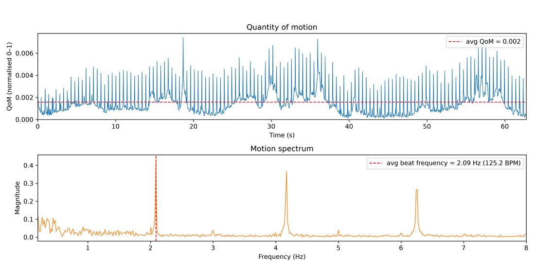Movement tempo: the quantity-of-motion signal and its FFT movement spectrum, with the dominant tempo marked.

Restrict the search band with fmin/fmax (Hz).

---

Motion descriptors

motiondescriptors() summarises how something moves with a compact set of higher-level scalar descriptors computed from the quantity-of-motion (QoM) signal — complementing the per-frame data from motion():

descriptor	meaning
motion_energy	mean squared QoM — the overall amount of movement.
motion_smoothness	SPARC (spectral arc length), a dimensionless, validated smoothness metric. It is non-positive; less negative = smoother, more negative = jerkier.
motion_entropy	normalised (0–1) Shannon entropy of the QoM magnitude distribution — the complexity/variedness of the motion.
dominant_freq	the main movement-rhythm rate (Hz) from the QoM power spectrum.
spectral_centroid	the "centre of mass" (Hz) of the movement spectrum.

md = mv.motiondescriptors()                 # returns MgFigure
print(md.data['motion_smoothness'])         # SPARC smoothness
print(md.data['motion_entropy'])            # 0–1
md.show()                                    # QoM time series + power spectrum

The spectral descriptors use a Hann window by default to reduce leakage from the finite QoM segment; pass window='none' for a rectangular window. The dominant frequency and spectral centroid are searched within a movement band (fmin/fmax, default 0.2–10 Hz) so slow amplitude drift near 0 Hz doesn't masquerade as the movement rhythm. The scalars are also written to a _motiondescriptors.csv (set save_data=False to skip), and data['frequencies']/data['power'] hold the full spectrum.

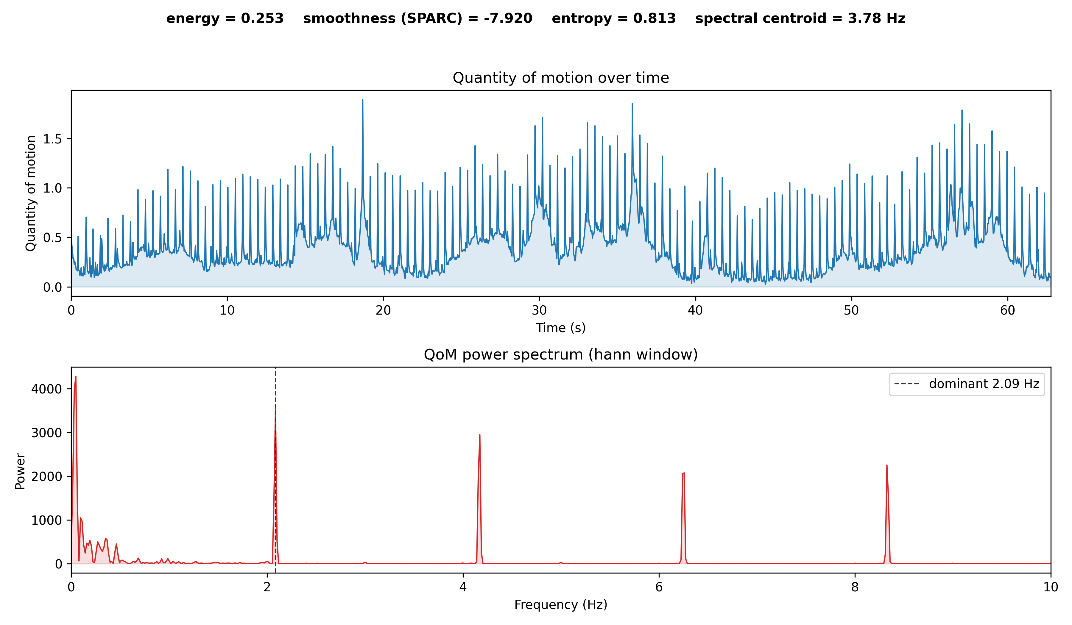Quantity of motion over time and its Hann-windowed power spectrum, with the dominant movement frequency marked; the energy / SPARC smoothness / entropy / spectral-centroid scalars are shown above.

---

Motion vectors

motionvectors() visualises the motion vectors carried by inter-frame codecs (MPEG, H.264, H.265) using FFmpeg's codecview filter — a decoder-level view of motion with no recomputation.

mvecs = mv.motionvectors()      # returns MgVideo
mvecs.show()

Per-block motion vectors drawn by the decoder's codecview filter.

Note

Intra-only formats (e.g. MJPEG in many .avi files) carry no motion vectors. Convert to an mp4/H.264 source first to see them.

---

Eulerian Video Magnification

eulerian() amplifies subtle changes that are normally invisible (Wu et al., SIGGRAPH 2012).

# Amplify subtle COLOUR changes (e.g. pulse, breathing)
evm = mv.eulerian(mode='color', freq_low=0.83, freq_high=1.0, amplification=50)

# Amplify subtle MOTION
evm = mv.eulerian(mode='motion', freq_low=0.4, freq_high=3.0, amplification=20)
evm.show()

Eulerian video magnification: subtle changes amplified across the output video.

• mode='color' uses a Gaussian pyramid + ideal FFT temporal band-pass (two-pass, low memory)
• mode='motion' uses a Laplacian pyramid + streaming IIR band-pass (frame-by-frame, low memory)
• freq_low/freq_high set the temporal band in Hz; amplification is the gain; levels the pyramid depth

---

Sonomotiongram

sonomotiongram() sonifies the motiongram: the motiongram matrix is treated as a magnitude spectrogram (spatial position → frequency, motion intensity → amplitude) and resynthesised to audio via an inverse STFT (Griffin–Lim). It returns an MgAudio, so you can analyse or play the result.

son = mv.sonomotiongram(sonogram='vertical')   # or 'horizontal' — returns MgAudio
son.waveform().show()
son.spectrogram().show()
# rendered WAV at son.filename

---

Videograms

Videograms apply the motiongram technique to the source video directly, without first computing frame differences. They show the full scene content over time rather than motion only.

videograms = mv.videograms()    # returns MgList[MgImage, MgImage]
videograms[0].show()            # horizontal videogram
videograms[1].show()            # vertical videogram
videograms.show(key='horizontal')
videograms.show(key='vertical')
mv.show(key='horizontal')
mv.show(key='vertical')

Horizontal videogram: the full scene content (not motion) collapsed onto the y-axis, flowing left→right over time.

Vertical videogram: the full scene content collapsed onto the x-axis, stacked top→bottom over time.

---

Self-Similarity Matrix (SSM)

SSMs compare each column or row of a motiongram or videogram against all others, revealing periodic structure in the motion.

motionssm = mv.ssm(features='motiongrams')              # returns MgList
motionssm = mv.ssm(features='motiongrams', cmap='viridis', norm=2)
motionssm[0].show()     # horizontal SSM
motionssm[1].show()     # vertical SSM
mv.show(key='ssm')

# both axes of motion in a single SSM (returns one MgImage)
combined = mv.ssm(features='motiongrams', combine=True)
combined.show()

videossm = mv.ssm(features='videograms')
chromassm = mv.ssm(features='chromagram', cmap='magma', norm=2)
spectrossm = mv.ssm(features='spectrogram')

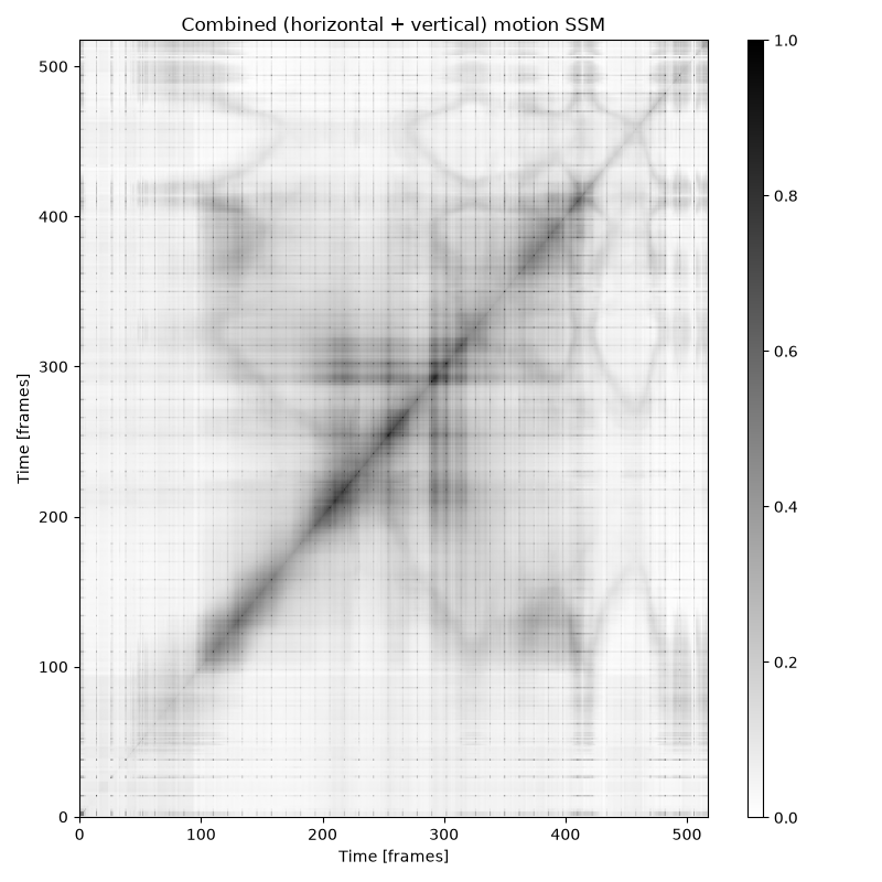Combined motion SSM: both axes of motion in a single self-similarity matrix, revealing periodic structure over time.

---

Background subtraction

subtract() removes a static background from each frame. If no background image is provided, it computes the frame average automatically.

subtraction = mv.subtract()                                             # returns MgVideo
subtraction = mv.subtract(bg_img='/path/to/background.png', bg_color='#ffffff')
subtraction = mv.subtract(bg_img='/path/to/background.png', curves=0.3)
subtraction.show()
mv.show(key='subtract')

---

Grid preview

grid() assembles a strip of evenly-spaced frames into a single image, useful for quickly reviewing a recording.

grid = mv.grid(height=300, rows=3, columns=3)  # returns MgImage
grid.show()
grid_array = mv.grid(height=300, rows=3, columns=3, return_array=True)

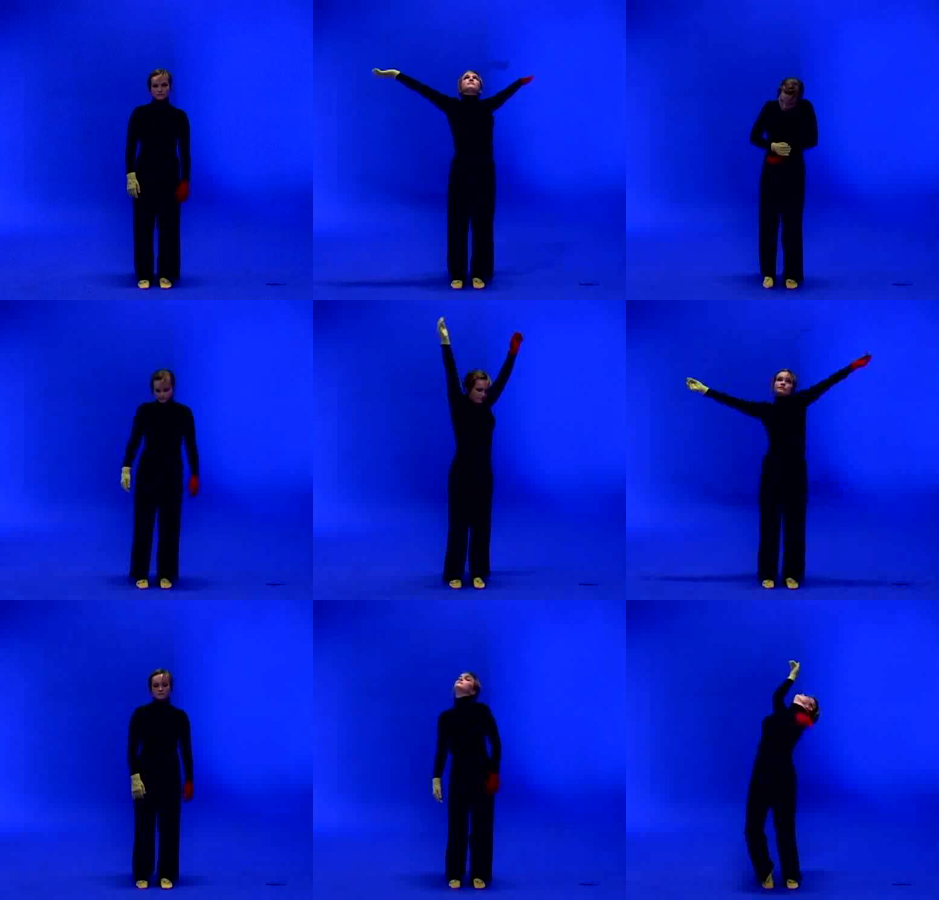Grid: a strip of evenly-spaced frames assembled into a single image for a quick overview of the recording.

---

History video

history() overlays the last history_length frames onto each frame, making the trajectory of motion visible.

history = mv.history(history_length=20)     # returns MgVideo
history.show()
mv.show(key='history')

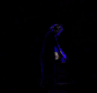History applied to a motion video: each frame overlays the last history_length frames, tracing the trajectory of motion.

Applying history to a motion video emphasises movement traces:

motionhistory = mv.motionvideo().history()
mv.show(key='motionhistory')

---

Blend

blend() combines all frames into a single image using a compositing mode.

average = mv.average()                          # returns MgImage (mean of all frames)
average = mv.blend(component_mode='average')    # equivalent
lighten = mv.blend(component_mode='lighten')
darken  = mv.blend(component_mode='darken')
average.show()
mv.show(key='blend')

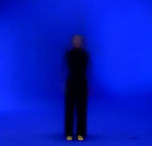Average: the pixel-wise mean of every frame — a long-exposure-style summary of the whole clip.

Motion average — blend applied to a motion video — shows where movement was concentrated:

motion_average = mv.motionvideo().blend(component_mode='average')
motion_average.show()

---

Pose estimation

pose() runs skeleton estimation on each frame, with two backends:

• MediaPipe (model='mediapipe', the default): Google MediaPipe Pose, 33 landmarks with depth and visibility. Fast on plain CPU, needs no CUDA-enabled OpenCV build, and works on the standard pip OpenCV (with optional GPU via MediaPipe's own delegate). Best for single-person analysis. Model weights auto-download (~8–28 MB) on first use.
• OpenPose (model='body_25'/'coco'/'mpi'): Caffe models (~200 MB on first use). Support multi-person analysis, but are slow without an OpenCV compiled with CUDA.

pose = mv.pose()                                                # MediaPipe by default
pose = mv.pose(device='gpu')                                    # MediaPipe with GPU delegate
pose = mv.pose(model='coco', device='cpu', downsampling_factor=4)   # OpenPose, multi-person
pose = mv.pose(model='body_25', device='gpu', threshold=0.1)
pose.show()
mv.show(key='pose')

# draw only the markers on a black background (no video underneath)
pose = mv.pose(style='markers', overlay=False)
# draw only the skeleton (joint lines) over the video
pose = mv.pose(style='skeleton')
# markers/skeleton on a white background (print-friendly: black skeleton + markers)
pose = mv.pose(overlay=False, background='white')
# leave a motion trail behind each marker over the last 10 frames
pose = mv.pose(marker_history=10)

• model: 'mediapipe' (default), 'body_25', 'coco', or 'mpi'
• style: 'both' (default), 'markers' (keypoints only), or 'skeleton' (joint lines only)
• overlay: True (draw on the video) or False (draw on a plain background)
• background: 'black' (default) or 'white' — the background colour when overlay=False. 'black' draws bright colours; 'white' draws a black skeleton and markers for a print-friendly inverted look.
• marker_history: 0 (default) draws nothing extra; when > 0, draws a motion trail for each marker by joining its positions over the last N frames. Works in all render paths.
• device: 'cpu' or 'gpu'. For OpenPose models, if device='gpu' is requested but OpenCV lacks CUDA, pose() automatically switches to the MediaPipe backend (when installed) so the GPU is still used; otherwise it falls back to CPU.
• downsampling_factor: reduces input resolution before inference (OpenPose only); higher is faster but less accurate
• threshold: minimum network confidence to accept a keypoint (normalised 0–1)
• data_format: 'csv' (default), 'tsv', 'txt', or 'c3d' (motion-capture format; needs the optional c3d package). Combine, e.g. data_format=['csv', 'c3d'].
• use_cache: reuse keypoints from a previous pose() run (same model/threshold) to re-render a different style/overlay/background without re-running inference — e.g. run style='markers' then style='skeleton' and the second call is near-instant. Defaults to True.

mv.pose(style='markers')      # runs inference, caches keypoints
mv.pose(style='skeleton')     # reuses cache — no re-inference
mv.pose(data_format=['csv', 'c3d'])   # also write a .c3d mocap file

pose() also renders two summary images of the whole video (disable with save_average_pose=False / save_trajectories=False), attached to the returned video:

pv = mv.pose()
pv.average_pose.show()     # markers coloured by normalised QoM, with per-marker "QoM | frequency" labels
pv.trajectories.show()     # every marker's spatial path over the whole video
# a per-marker stats CSV (<name>_pose_average_stats.csv) with normalised QoM and frequency is also saved

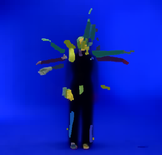
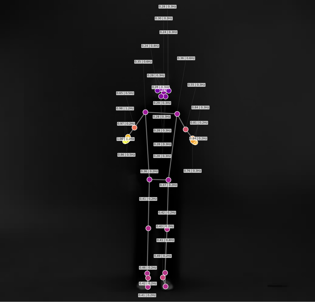Average pose: markers placed at their mean position, coloured by normalised quantity of motion and annotated with a QoM | frequency label (no colorbar, no title).

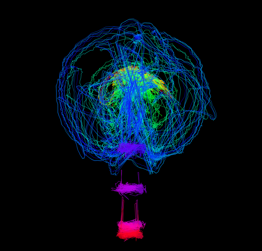Marker trajectories: every marker's spatial path over the whole video. The background follows trajectory_background (default 'black').

Both summary images are decluttered: neither carries an in-figure title. The average-pose image no longer draws a colorbar — markers are still coloured by quantity of motion, and each one is annotated with a QoM | frequency number label (normalised QoM 0–1 and dominant frequency in Hz). These labels are automatically laid out so they don't overlap (with thin leader lines back to each marker). The marker-trajectories image shows no per-marker name labels by default (trajectory_labels=False); re-enable them with trajectory_labels=True.

Control the trajectories image background with trajectory_background: 'black' (default), 'white', or 'transparent' (so you can overlay the paths on the video afterwards). This supersedes the older transparent_trajectories flag, which is still accepted.

mv.pose(trajectory_background='transparent')   # paths on a transparent PNG for overlay
mv.pose(trajectory_background='white')         # print-friendly white background
mv.pose(trajectory_labels=True)                # show marker names on the trajectories image
mv.pose(transparent_trajectories=True)         # legacy flag, still accepted

GPU acceleration

pose(model='mediapipe', device='gpu') gives GPU acceleration with the standard pip OpenCV. The OpenCV-based methods (flow.dense(use_gpu=True), blur_faces(use_gpu=True), OpenPose device='gpu') need an OpenCV built with CUDA. Use mg.cuda_build_available() to check, and mg.cuda_unavailable_reason() for an explanation.

Pose waterfall

pose_waterfall() renders a 3D spatio-temporal waterfall where each pose marker's trajectory flows through (x, time, y) space — a pose-based counterpart to silhouette_waterfall(). It returns an MgFigure. It reuses cached pose keypoints from a prior pose() call; otherwise it runs pose() first (pose kwargs like model/device are forwarded).

wf = mv.pose_waterfall()                       # returns MgFigure ('trajectories' style)
wf = mv.pose_waterfall(color_by='time')        # colour follows time along each path
wf = mv.pose_waterfall(markers=['left_wrist', 'right_wrist'], cmap='viridis')
wf = mv.pose_waterfall(style='skeleton')       # skeleton joint lines at sampled time slices
wf = mv.pose_waterfall(style='markers', n_samples=60)
wf = mv.pose_waterfall(axes=False)             # clean render, no axes/labels
wf = mv.pose_waterfall(crop=True)              # tighten to the data, trim whitespace
wf.show()

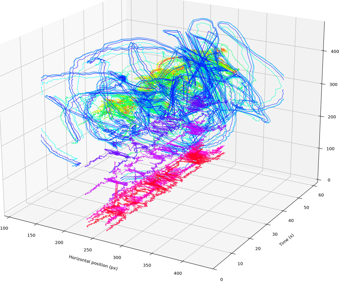
style='trajectories': each marker's continuous path flowing through (x, time, y) space.

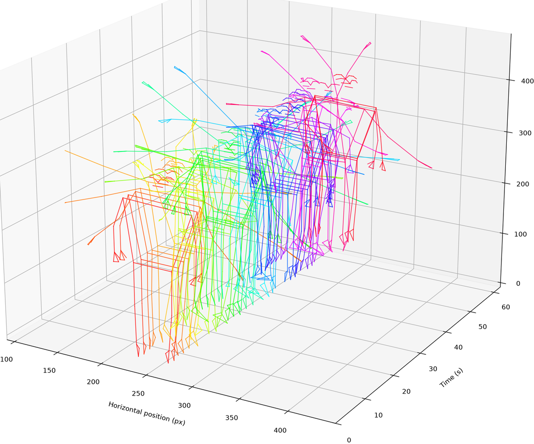
style='skeleton': the skeleton joint lines drawn at n_samples time slices, coloured by time.

• style: how the waterfall is drawn —
  • 'trajectories' (default): continuous per-marker paths flowing through (x, time, y) space
  • 'markers': markers scattered at discrete time slices
  • 'skeleton': skeleton joint lines drawn per time slice
  • 'both': markers and skeleton lines together

The slice-based styles ('markers', 'skeleton', 'both') sample n_samples time slices (default 40) and default to colour-by-time. - markers: which markers to plot (default None = all) - color_by: 'marker' (one colour per marker) or 'time' (colour follows time). Defaults to 'marker' for 'trajectories' and to 'time' for the slice styles. - cmap: matplotlib colormap ('hsv' default); dpi (default 200); lw line width (default 1.0) - elev/azim: 3D view angles (defaults 20 / -60) - axes: set to False to render without any axes, ticks, labels, or panes (a clean 3D image). Defaults to True. (silhouette_waterfall() accepts the same axes option.) - crop: set to True to tighten the spatial limits to the marker extent and trim the surrounding whitespace, so the figure shows mostly the data. Defaults to False. - plus the usual target_name, overwrite, and forwarded **pose_kwargs (e.g. model, device)

Pose segments (circular statistics)

pose_segments() analyses each body segment — the bone between two connected joints (e.g. shoulder→elbow) — and draws a grid of circular (polar rose) plots, one per segment. For each segment it computes the per-frame orientation angle and shows a rose histogram of the angle distribution with the mean-direction resultant vector. It returns an MgFigure and saves a per-segment statistics CSV. Like pose_waterfall(), it reuses cached pose keypoints from a prior pose() call, otherwise runs pose() first (pose kwargs are forwarded).

seg = mv.pose_segments()                       # returns MgFigure ('viridis' roses)
seg = mv.pose_segments(n_bins=24, cmap='magma', ncols=4)
seg = mv.pose_segments(segments=[(11, 13), (13, 15)])   # only chosen joint pairs
seg.show()

stats = seg.data['stats']                      # per-segment circular statistics

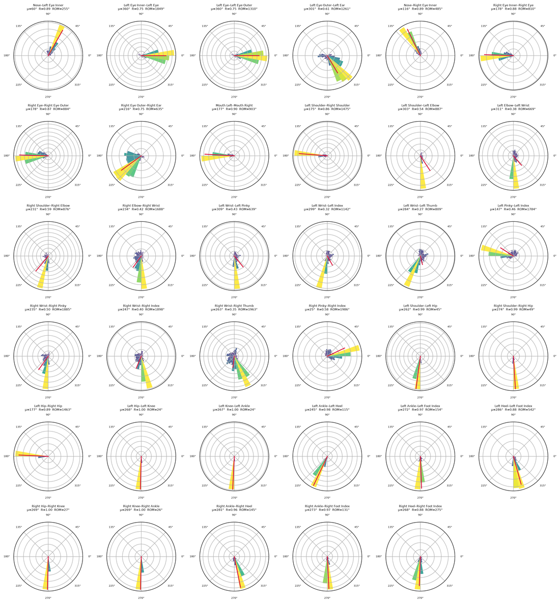Per-segment polar rose plots: the angular distribution of each bone's orientation, with the mean-direction resultant vector.

The saved CSV (and seg.data['stats']) reports, per segment: mean angle, resultant length R (0–1, concentration of direction), circular standard deviation, range of motion, and mean angular speed.

• segments: list of (a, b) joint-index tuples to restrict the analysis (default None = all skeleton connections)
• n_bins: angular bins per rose (default 36 = 10° bins)
• cmap: colormap for the bars ('viridis' default); ncols sets the subplot-grid width (default 6); dpi (default 200)
• plus the usual target_name, overwrite, and forwarded **pose_kwargs

Pose centring

pose_center() centres the pose data on its global centroid — a 2D port of the MoCap Toolbox mccenter. A single offset per coordinate (the mean of the per-marker temporal means, missing detections ignored) is subtracted from every marker so the overall spatiotemporal centroid sits at the origin. This removes the performer's absolute position in the frame, leaving relative posture/movement — useful before comparing or further analysing trajectories. It plots the centred marker trajectories, saves a CSV of the centred coordinates, and returns an MgFigure (the centred (T, n, 2) array is in .data['coords'], the removed offset in .data['offset']).

pc = mv.pose_center()          # returns MgFigure (+ CSV); reuses cached keypoints or runs pose()
pc.show()
centred = pc.data['coords']    # (frames, markers, 2), centroid at the origin

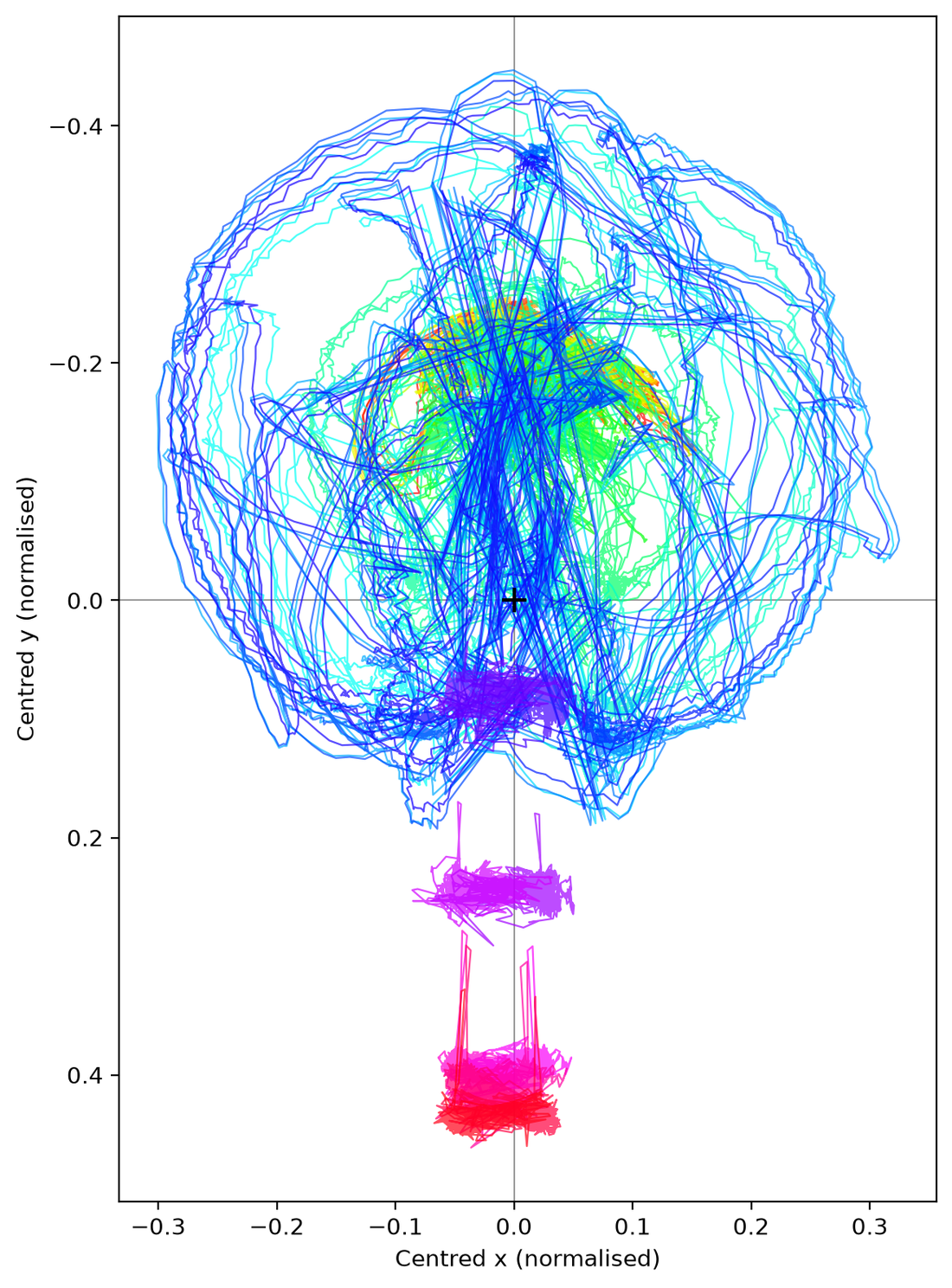Each marker's trajectory after centring on the global centroid (origin marked).

Distance travelled

pose_distance() computes each marker's cumulative distance travelled (the sum of frame-to-frame Euclidean displacement, in pixels) plus the across-marker average — a 2D port of mccumdist. The figure shows the per-marker cumulative-distance curves and a ranked total-per-marker bar chart with the average marked; a CSV of the totals (and the average) is saved. .data holds total (per marker), average, and cumulative (the per-marker curves).

pd_fig = mv.pose_distance()    # returns MgFigure (+ CSV)
pd_fig.show()
print(pd_fig.data['average'])  # mean distance travelled across markers (px)

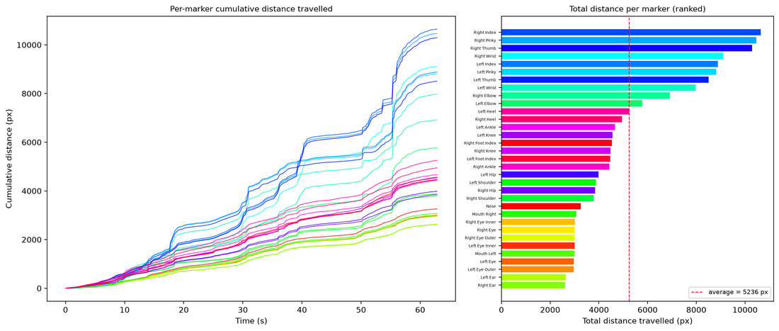Left: cumulative distance travelled per marker over time. Right: total per marker, ranked, with the across-marker average.

---

Audio–movement analysis

MGT-python provides a suite of reports that compare a single performer's sound with their movement — tempo similarity, phase synchrony, structural similarity, per-body-part coupling, and loudness-vs-motion dynamics coupling — alongside the sonification and beat-warping tools. These now have their own page:

➡️ Audio-Video Processing & Analysis

mv.tempo_similarity().show()      # audio tempo vs movement tempo
mv.phase_synchrony().show()       # phase-locking value (PLV)
mv.structure_comparison().show()  # audio SSM vs movement SSM + difference
mv.body_audio_coupling().show()   # which body parts track the music
mv.dynamics_coupling().show()     # audio loudness vs quantity of motion

---

Optical flow

Sparse

Sparse optical flow tracks a small set of salient feature points and draws their trajectories.

flow_sparse = mv.flow.sparse()      # returns MgVideo
flow_sparse.show()
mv.show(key='sparse')

Sparse optical flow: tracked feature points and their trajectories.

Dense

Dense optical flow estimates movement at every pixel, colour-coding direction.

flow_dense = mv.flow.dense()                    # returns MgVideo
flow_dense = mv.flow.dense(use_gpu=True)        # CUDA acceleration with CPU fallback
flow_dense.show()
mv.show(key='dense')

Dense optical flow: hue encodes direction, brightness encodes speed, at every pixel.

Velocity

Setting velocity=True computes per-frame speed instead of direction, and returns an MgFigure with the velocity plot and associated data.

velocity = mv.flow.dense(velocity=True)
velocity_per_meters = mv.flow.dense(velocity=True, distance=3.5, angle_of_view=80)
xvel = velocity.data['xvel']
yvel = velocity.data['yvel']
velocity.figure

---

Face anonymisation

blur_faces() detects faces in every frame and applies a blur, black rectangle, or image mask.

blur = mv.blur_faces()                                  # returns MgVideo
blur = mv.blur_faces(use_gpu=True)
blur = mv.blur_faces(save_data=True, data_format='csv')
blur.show()
mv.show(key='blur')

source_image = '/path/to/mask.jpg'
mv.blur_faces(mask='image', mask_image=source_image)

To render a heatmap of face detection centroids instead:

heatmap = mv.blur_faces(draw_heatmap=True, neighbours=128, resolution=500, save_data=False)
heatmap.show()

---

Warp audiovisual beats

warp_audiovisual_beats() temporally aligns visual beats (extracted from directograms) with audio beats to create a re-timed video.

warp = mv.warp_audiovisual_beats('/path/to/audio.wav')  # returns MgVideo
warp.show()
mv.show(key='warp')

Directograms

Directograms factor motion magnitude into angular bins, analogous to a spectrogram with angles replacing frequencies.

directograms = mv.directograms()    # returns MgFigure
directograms.data['directogram']
directograms.show()

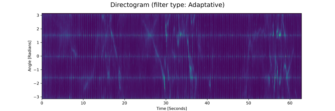Directogram: motion magnitude factored into angular bins over time, like a spectrogram with angles replacing frequencies.

Impacts

Impacts are visual analogues of audio onset envelopes, derived from directogram deceleration.

impacts = mv.impacts(detection=False)                               # returns MgFigure
impacts = mv.impacts(detection=True, local_mean=0.1, local_maxima=0.15)
impacts.data['impact envelopes']
impacts.show()

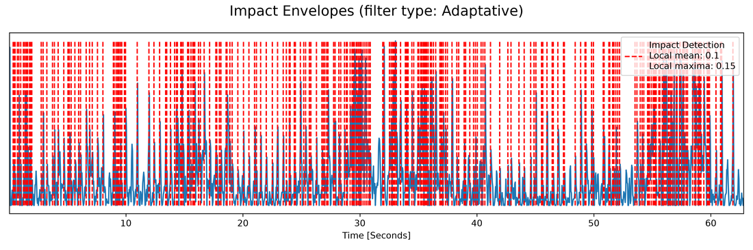Impacts: the visual onset envelope derived from directogram deceleration, the movement analogue of an audio onset envelope.

---

Next steps

• Audio Analysis — waveforms, spectrograms, and audio features
• Working with Results — combining and displaying MgFigure, MgImage, and MgList
• API Reference — complete motion method signatures