Audio-Video Processing & Analysis¶

MGT-python treats sound and movement as two views of the same performance. This page collects the tools that cross the two domains — converting between them, aligning them, and measuring how similar a performer's movement is to the sound they make. They are especially useful for studying a single dancer who is also the sound source.

All methods below are called on an MgVideo:

import musicalgestures as mg
mv = mg.MgVideo('/path/to/video.avi')

The analysis methods require the video to have an audio track and return an MgFigure (numeric results in .data); most also save a CSV next to the image.

Audio–video processing¶

These methods convert or re-time across the two domains.

Sonification (motion → sound)¶

sonomotiongram() sonifies the motiongram: the motiongram matrix is treated as a magnitude spectrogram (spatial position → frequency, motion intensity → amplitude) and resynthesised to audio via an inverse STFT (Griffin–Lim). It returns an MgAudio, so you can analyse or play the result.

son = mv.sonomotiongram(sonogram='vertical')   # or 'horizontal' — returns MgAudio
son.waveform().show()
son.spectrogram().show()
# rendered WAV at son.filename

Beat-aligned video (warp)¶

warp_audiovisual_beats() temporally aligns the visual beats (extracted from directograms) with the audio beats to produce a re-timed video in which movement and music fall together.

warp = mv.warp_audiovisual_beats('/path/to/audio.wav')  # returns MgVideo
warp.show()

Audio–movement analysis¶

These reports estimate an audio envelope and a movement envelope from the same clip and compare them, quantifying how similar the sound and the movement are.

Tempo similarity¶

tempo_similarity() compares the audio tempo (from the onset-strength envelope) with the movement tempo (from the quantity-of-motion envelope). The two-panel figure overlays the normalised envelopes and shows their cross-correlation; the report lists audio BPM, movement BPM, their ratio and nearest harmonic relationship, the peak cross-correlation and its lag, and the zero-lag correlation.

ts = mv.tempo_similarity()                     # returns MgFigure (+ CSV)
ts.show()
print(ts.data['audio_tempo_bpm'], ts.data['motion_tempo_bpm'])
print(ts.data['tempo_ratio'], ts.data['nearest_harmonic'])

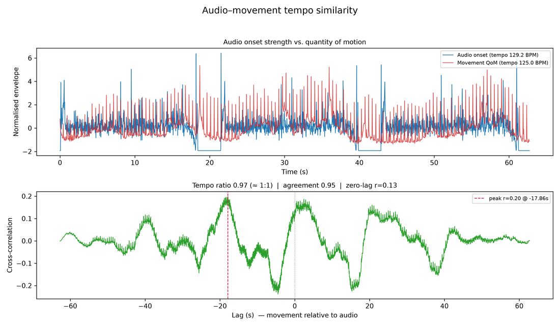Audio–movement tempo similarity of dance.avi Top: audio onset strength vs. quantity of motion. Bottom: their cross-correlation, with the peak lag and tempo ratio annotated.

Phase synchrony¶

phase_synchrony() band-passes both the audio onset envelope and the movement QoM to the tempo band [fmin, fmax] Hz and compares their instantaneous phases (Hilbert transform). It reports the phase-locking value (PLV, 0–1: how consistent the audio↔movement phase difference is) and draws a polar histogram of the phase difference.

ps = mv.phase_synchrony(fmin=0.5, fmax=4.0)    # returns MgFigure
ps.show()
print(ps.data)                                 # PLV, mean phase difference, …

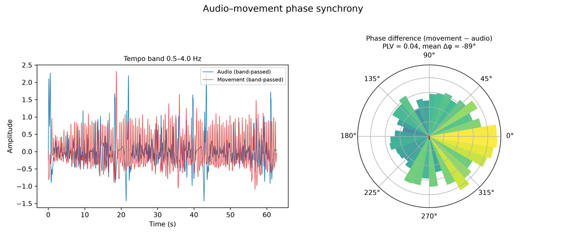Audio–movement phase synchrony of dance.avi Left: the band-passed audio and movement signals. Right: a polar histogram of the phase difference with the PLV.

Structure comparison¶

structure_comparison() builds a self-similarity matrix (SSM) of the audio (from MFCC frames) and of the movement (from low-resolution frame appearance), resampled to the same number of time points, and shows them side by side with their absolute difference map. Bright regions in the difference are where the musical structure and the movement structure diverge; it reports an overall structural-agreement score.

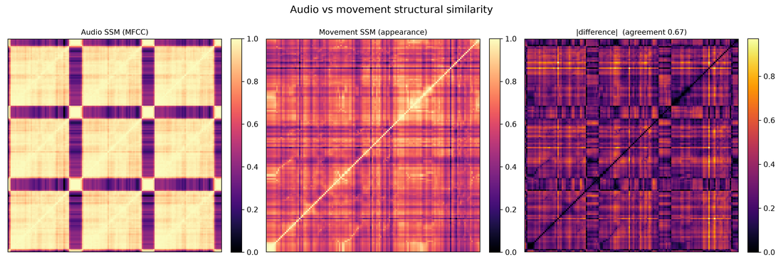sc = mv.structure_comparison(n=200, cmap='magma')   # returns MgFigure
sc.show()

Audio vs. movement structure comparison of dance.avi Audio SSM (MFCC) vs. movement SSM (frame appearance) and their absolute difference.

Body–audio coupling¶

body_audio_coupling() correlates each pose marker's speed with the audio onset envelope, revealing which body parts are most rhythmically tied to the music. The figure shows a body map (the average pose with markers coloured by correlation) plus a ranked bar chart, and a CSV of per-marker correlations. It reuses cached pose keypoints or runs pose() first (pose kwargs forwarded).

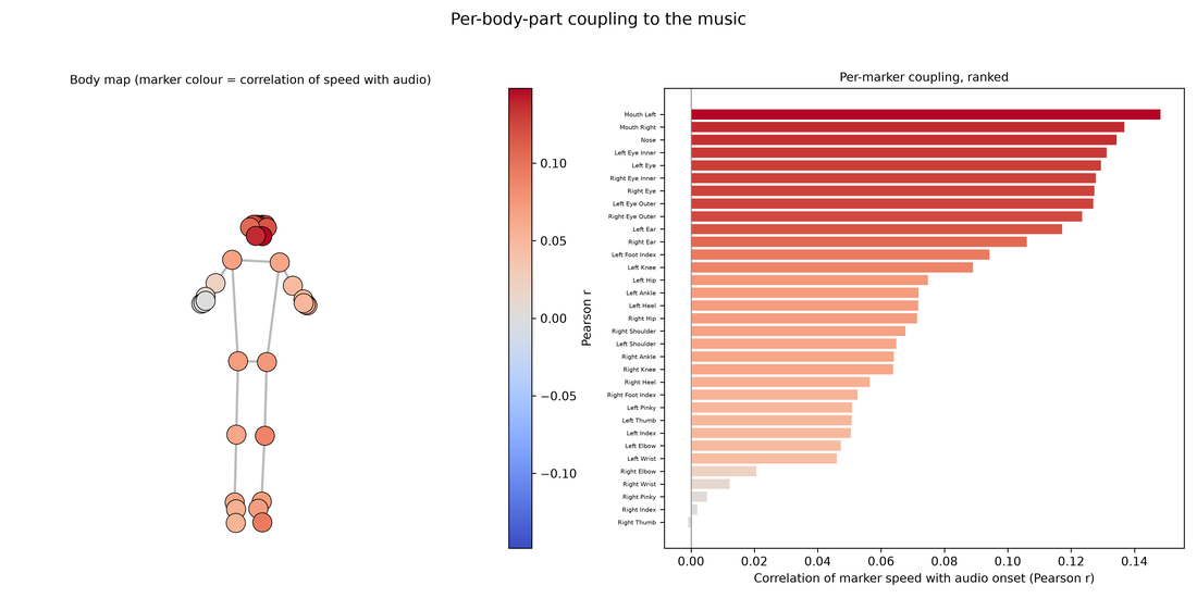bc = mv.body_audio_coupling(cmap='coolwarm')   # returns MgFigure (+ CSV)
bc.show()

Per-body-part audio coupling of dance.avi Each marker coloured by how strongly its speed correlates with the audio onset envelope, plus a ranked bar chart.

Dynamics coupling¶

dynamics_coupling() compares audio loudness (RMS) with movement quantity (QoM) — does the performer move more when the music is louder? It aligns the two envelopes and reports their correlation at zero lag and at the best lag within max_lag seconds; the figure overlays the normalised envelopes and shows a loudness-vs-motion scatter.

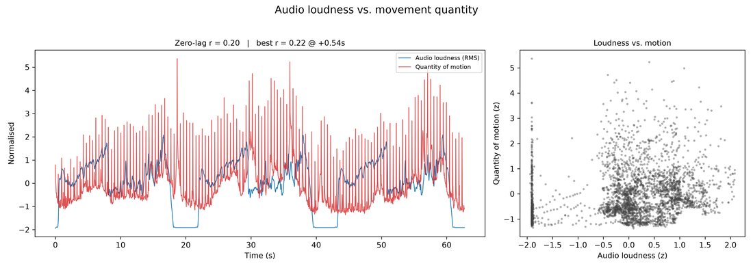dc = mv.dynamics_coupling(max_lag=2.0)         # returns MgFigure
dc.show()

Audio loudness vs. movement quantity coupling of dance.avi Audio RMS loudness overlaid on quantity of motion, with the loudness-vs-motion scatter and correlation.

These analyse rhythm within one domain but are natural companions to the comparisons above:

beat_statistics(source='motion') — circular timing statistics of the movement beats (use source='audio' for the audio track). See Audio Analysis.
motiontempo() — dominant movement tempo (Hz/BPM) from the quantity-of-motion spectrum. See Video Analysis.
tempogram() / tempo() — audio tempo and beat tracking. See Audio Analysis.