Week 6: Harmony and melody

Last week, we explored the importance of timing and rhythm in sound and music. This week, our focus shifts to how frequencies interact both “horizontally” and “vertically.” Horizontal organization of frequencies gives rise to melodies; sequences of pitches unfolding over time, often shaped by rhythmic patterns. Vertical organization, on the other hand, leads to the formation of intervals, harmonies, and textures, as multiple pitches sound together or overlap. Understanding these dimensions is essential for analyzing how music conveys structure, emotion, and complexity. First, however, we need to define the concept of “tone”.

Tones¶

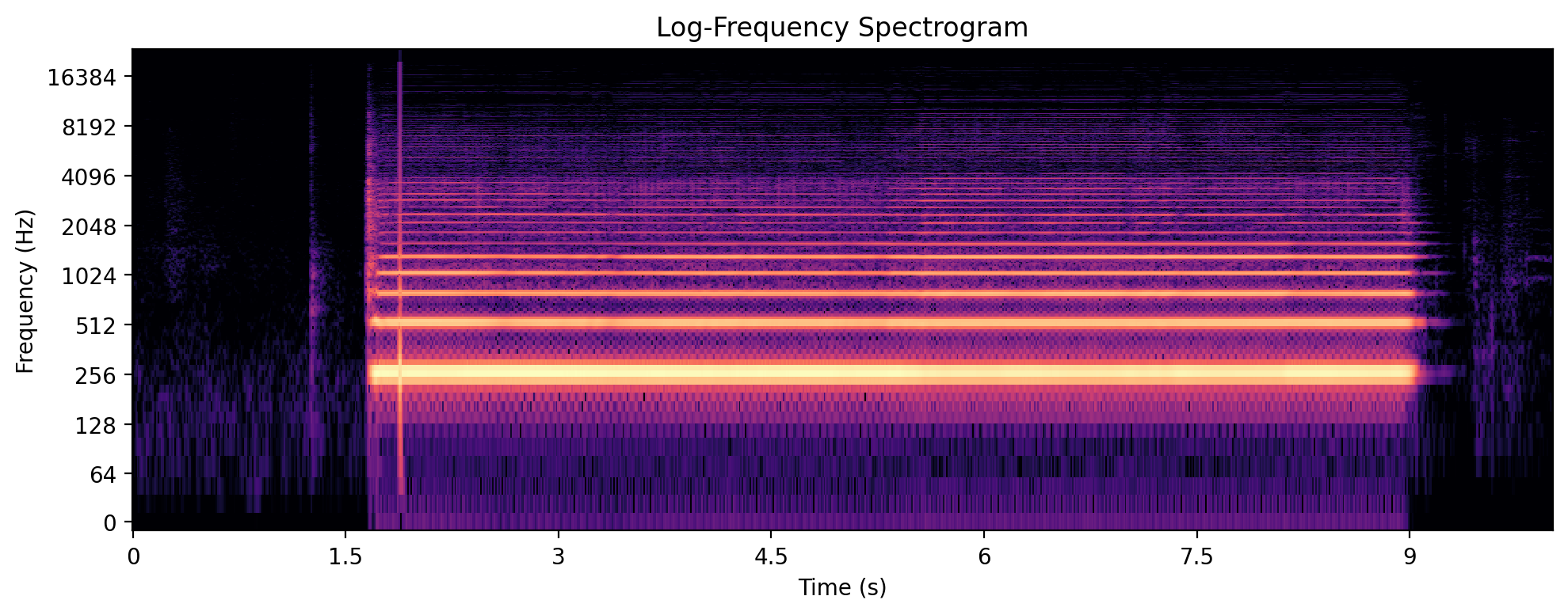
In music psychology, a tone is understood as a sound with a specific frequency, timbral quality, and temporal shape that the auditory system interprets as having a definite pitch. Our perception of tones is shaped by both the physical properties of the sound wave (such as frequency, amplitude, and harmonic content) and the way our brains process these signals. Tones are the building blocks of musical perception, allowing us to distinguish melodies, harmonies, and textures.

From a technical perspective, tones can be generated, analyzed, and manipulated using digital tools. Synthesizers create tones by combining waveforms, while audio analysis software can extract pitch and timbre features from recordings. Technologies such as pitch detection algorithms and spectral analysis are essential for applications in music information retrieval, automatic transcription, and digital instrument design.

Pitch¶

Pitch is the psycho-physiological correlate of frequency that lets us hear one sound as higher or lower than another. It is closely related to the fundamental frequency of a tone, but the relationship is not one-to-one. As you may recall from the Acoustics chapter, most instrument tones are not pure sine waves. Musical, “pitched” instruments generally produce a fundamental frequency (often abbreviated f0), which defines the perceived pitch. Additional overtones define the timbre of the instrument. Many musical instruments have overtones that are in a “harmonic” relationship to the fundamental frequency (f1, f2, etc.). For a tone with a fundamental frequency of 220 Hz, the harmonic overtones—sometimes called partials—are 440 Hz, 660 Hz, 880 Hz, etc. Interestingly, the individual partials of a complex sound are typically not perceived as separate; our perceptual system fuses them together, leading us to experience a unitary sound.

The pitch of harmonic tones generally corresponds to the fundamental frequency (f0). However, the brain can infer a fundamental frequency (and thus perceive pitch) from complex tones even when a fundamental component is absent. This is called "virtual pitch or the missing fundamental and it is related to the phenomenon whereby one’s brain extracts tones from everyday signals, even if parts of the signal are masked by other sounds.

Below is a sequence of simple (sine) tones distinct at different frequencies.

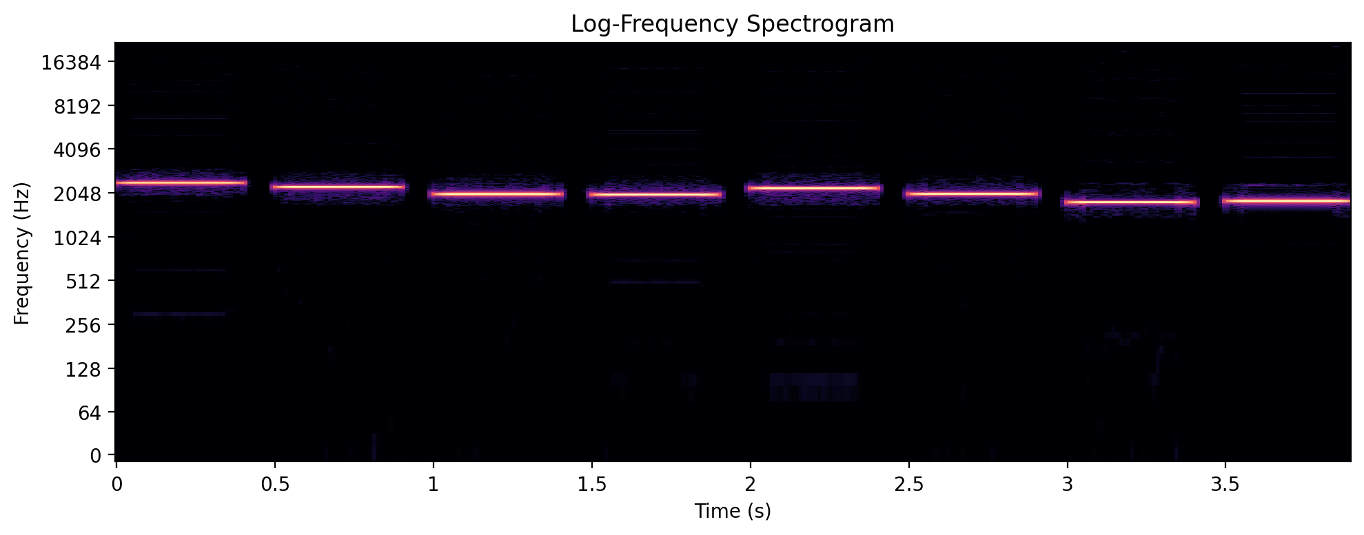
If we add some partials (multiples) below each tone, can you start to hear a familiar melody?

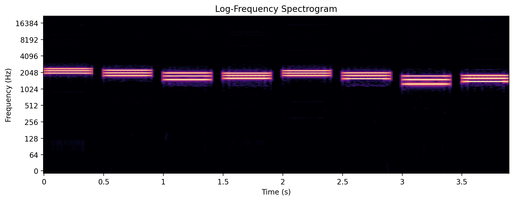
If we then rearrange these partials slightly, we can induce an even stronger sense of virtual pitch—various missing fundamental frequencies which are not physically present in the tones themselves:

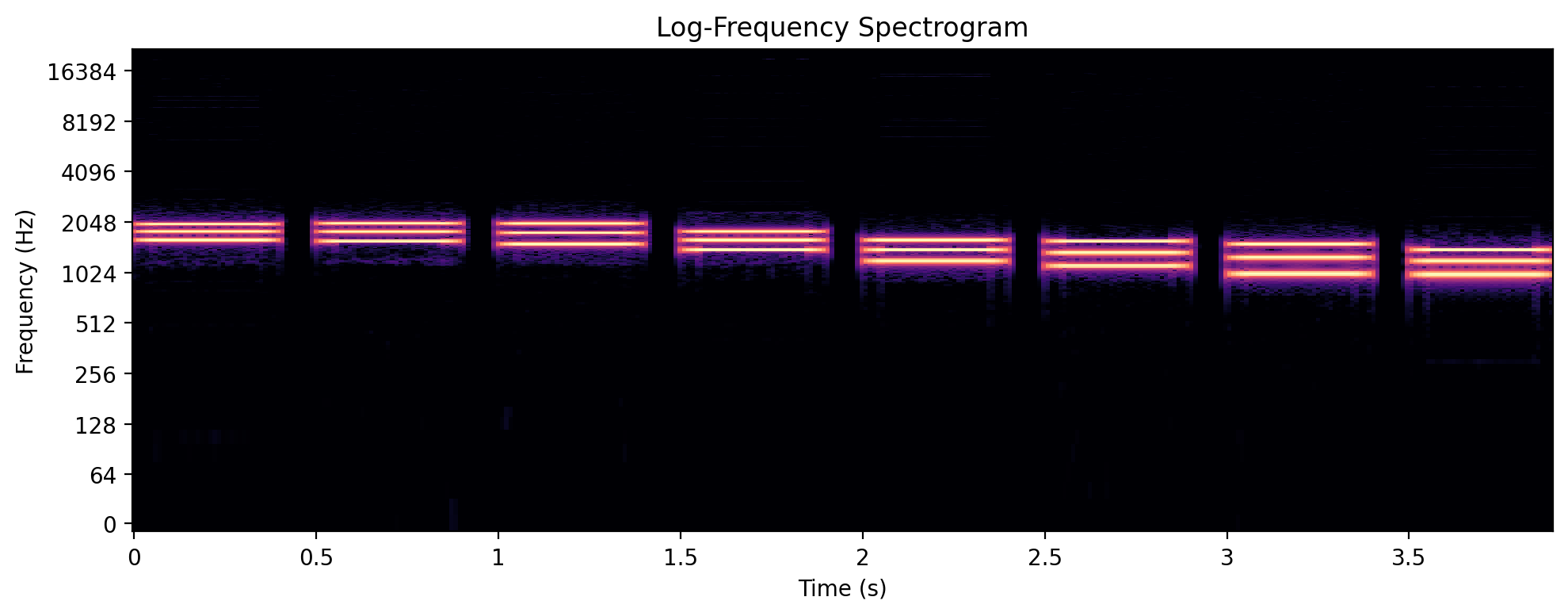
What happens is that your brain creates a virtual fundamental based on “calculating” the underlying frequencies part of the harmonic series.

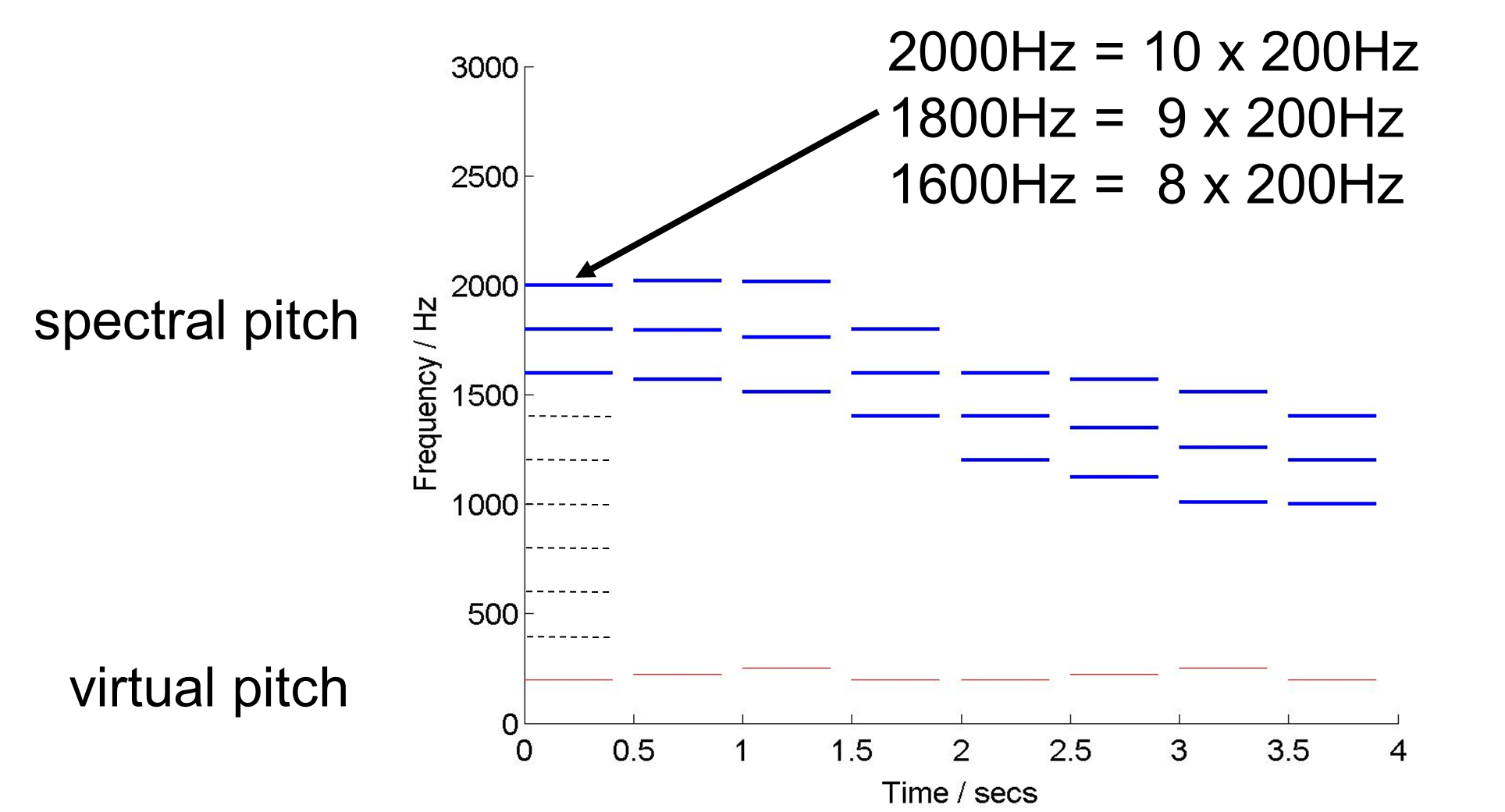
Image source: Toiviainen, P. (2015). Lecture materials for Music Perception. University of Jyväskylä.

Constant-Q Transform¶

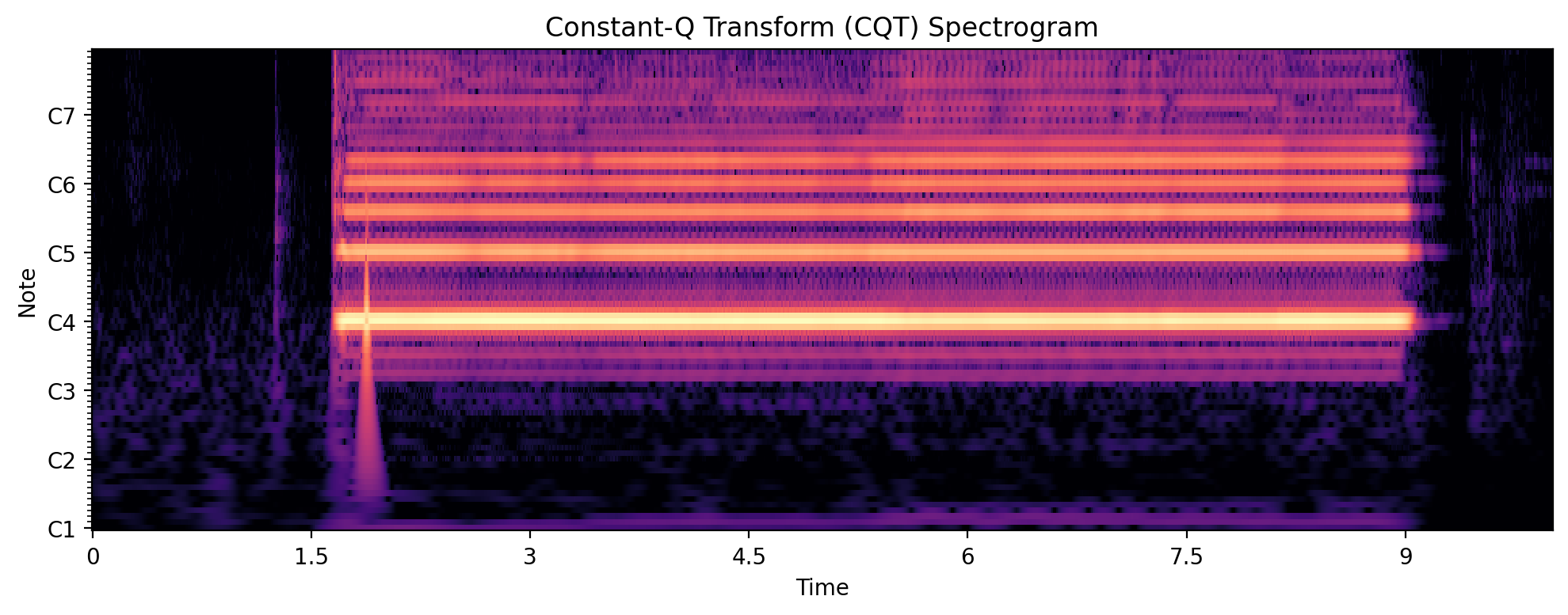
Up until now, we have looked at regular spectrograms, both linear and logarithmic. Both have their benefits, but generally, the logarithmic better represents human hearing. To analyze pitch, however, it is often better to use the constant-Q transform (CQT), a spectral analysis method that maps frequencies to musical notes. Unlike the standard spectrogram, which uses a linear frequency scale, the CQT uses a logarithmic scale that aligns with how musical notes are spaced, where each octave is divided into equal steps. This makes it easier to identify which pitch classes are present in a sound and is especially useful for tasks like chord recognition, key detection, and melody analysis.

Musical notes are typically “imperfect” because they contain a rich set of overtones and partials that are not perfectly harmonic. In a CQT spectrogram, this complexity appears as energy spread across multiple frequency bins, not just at the fundamental frequency. This allows us to visualize both the main pitches and their harmonic content, providing deeper insight into the timbre and structure of musical sounds.

Pitch class¶

In music, a pitch class is a set of pitches that are a whole number of octaves apart, e.g., the pitch class C consists of the Cs in all octaves. Humans perceive the notes in a tonal scale as repeating once per octave. This provides the basis for producing and perceiving melodic patterns based on relative pitch relationships, that is, relative to a pitch class. Absolute pitch ability, on the other hand, is the ability to recognize (or reproduce) specific pitches without the help of a reference pitch and pitch class.

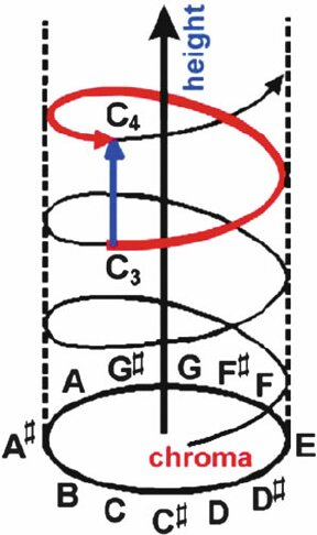
Image Source: Trainor, Laurel & Unrau, A.J.. (2012). Development of pitch and music perception. Springer Handbook of Auditory Research: Human Auditory Development. 223-254.

Chromagram¶

A chromagram visualizes the intensity of each of the 12 pitch classes (C, C#, D, ..., B) over time, regardless of octave. Below is a chromagram of the saxophone tone used above. Notice how the algorithm is less certain during the noisy attack and release portions, but clearly identifies the main pitch (C) during the sustained part of the tone. The presence of energy in the fifth (G) and third (E) pitch classes reflects their harmonic relationship to the tonic (C). Chromagrams are useful for analyzing harmonic and melodic content in music, as they abstract away octave information and focus on pitch class structure.

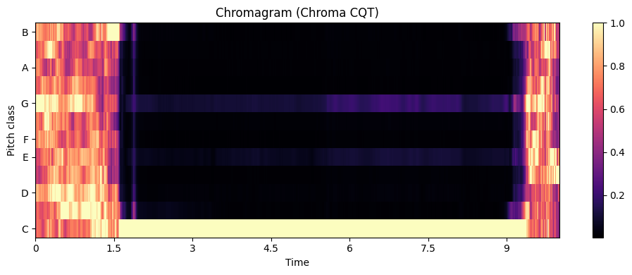
Tonality and Harmonic Expectation¶

Tonality is the organization of pitches and chords around a central note called the tonic, creating a sense of hierarchy and resolution in music. In Western music, tonality underlies the concept of key signatures (e.g., “C major”, “A minor”), where certain notes and chords feel stable (restful) while others create tension and seek resolution. This hierarchy is learned implicitly through exposure to music, forming a cognitive schema that shapes our expectations of which notes or chords will follow. Tonality is also supported by acoustics: the most important notes in a scale, such as the third and fifth, share harmonic overtones with the tonic, reinforcing their sense of belonging. Even without formal music theory training, listeners develop an intuitive sense of tonality and harmonic expectation through cultural experience.

Harmony¶

Harmony involves the combination of discernible tones to create intervals and chords. It is the simultaneous sounding of different pitches, which can evoke a wide range of emotional responses. Harmony plays a crucial role in the emotional tone and complexity of music. Harmony encompasses the interaction of pitches through intervals and chords, shaped by timbre and texture.

Intervals¶

An interval is the distance between two pitches, measured in steps or frequency ratios. Intervals are the building blocks of harmony, as they define the relationships between notes played together or in succession. In Western music theory, intervals are named by counting the number of letter names from the lower to the higher note (e.g., C to E is a third). They can be major, minor, perfect, augmented, or diminished.

The human brain is sensitive to the relationships between pitches, perceiving certain combinations as consonant (pleasant or stable) and others as dissonant (tense or unstable). For example, some intervals, like octaves and perfect fifths, are perceived as consonant, while others, like minor seconds or tritones, are more dissonant. These perceptual responses are influenced by cultural exposure, musical training, and innate auditory processing mechanisms.

Intervals form the basis for chords and harmonic progressions. The combination of intervals within a chord determines its character and function.

Chords¶

A chord is a group of three or more notes played simultaneously. Chords are the foundation of Western harmony and are used to create progressions that define the structure and mood of a piece.

Triads are the most basic chords, consisting of three notes (root, third, fifth). Types include major, minor, diminished, and augmented triads.

More complex chords can be created by adding additional notes, such as sevenths, ninths, elevenths, and thirteenths, which creates richer harmonies.

When combined, chords can create progressions that create movement and tension-resolution patterns in music (e.g., I–IV–V–I in classical music, or ii–V–I in jazz). In functional analysis, chords are defined by their roles (tonic, dominant, subdominant) and guide the listener’s expectations.

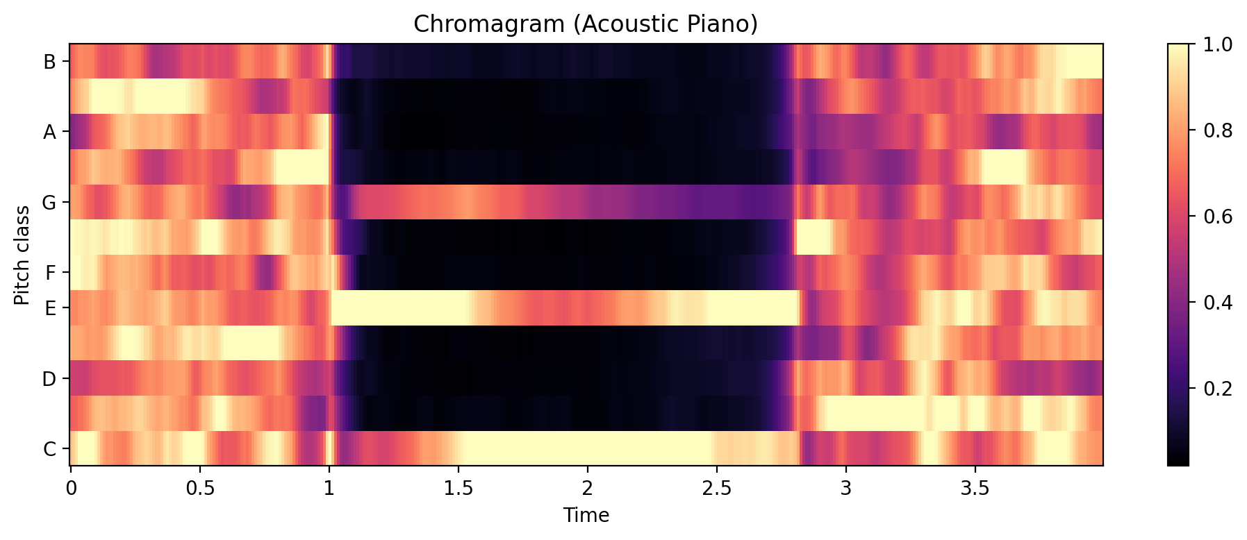
One of the reasons it is interesting to study music theory from the perspectives of psychology and technology is that the idealized concepts theorized in Western art music rarely exist in real life. For example, even a simple triad played on an acoustic piano exhibits rich timbral complexity, as you can both hear and see in the example below. Real-world sounds are shaped by the instrument’s physical properties, performance nuances, and acoustic environment, resulting in harmonic overtones and spectral features that go far beyond the abstract “perfect” chords described in theory. This highlights the importance of analyzing actual audio signals to understand how musical structures are perceived and experienced.

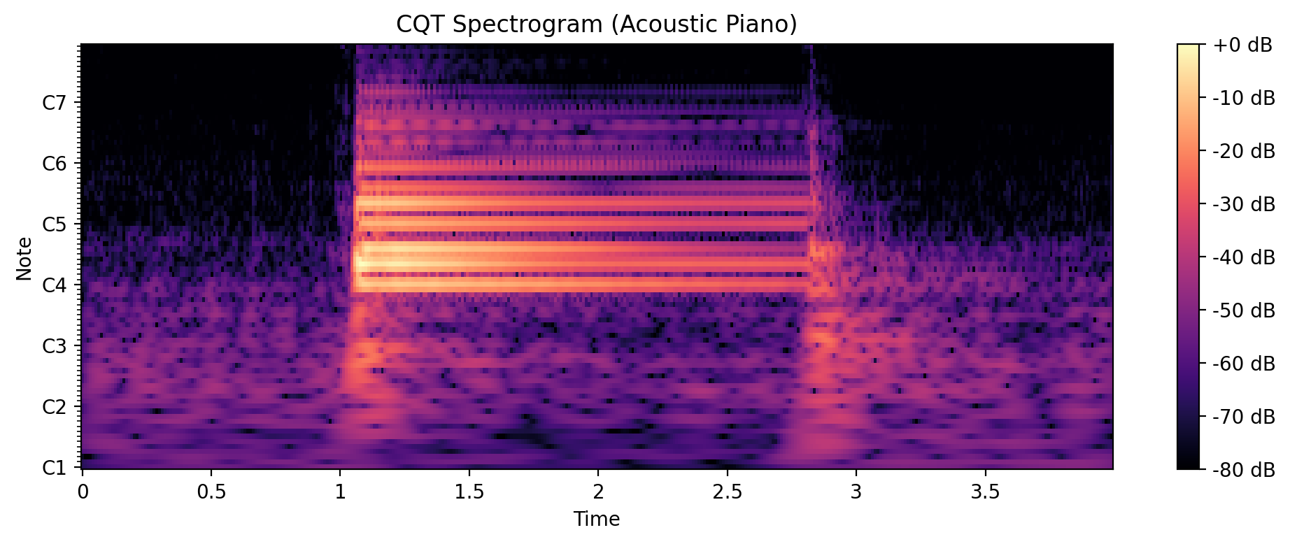
Melody¶

Melody is a sequence of musical notes perceived as a coherent whole. It is often the most recognizable and memorable aspect of a musical piece, playing a central role in emotional engagement and memory recall.

From a psychological perspective, melody is the perception of an organized sequence of tones that form a distinct musical line. The brain tracks pitch contours, intervals, and rhythmic patterns to identify, segment, and remember melodies. This ability underlies our capacity to recognize tunes, anticipate musical phrases, and experience emotional responses to music.

Technological advances have enabled detailed analysis and manipulation of melody. Pitch tracking algorithms can extract melodic lines from audio recordings, while MIDI editors and notation software allow for precise editing and visualization. In music generation and AI composition, models learn melodic patterns from large datasets to create new, stylistically consistent melodies. Melody extraction and similarity algorithms are also used in music search, recommendation systems, and music information retrieval.

Auditory scene analysis¶

Auditory scene analysis is the process by which the human auditory system organizes complex mixtures of sounds into perceptually meaningful elements, or “streams.” In music, this allows listeners to distinguish between different melodic lines, instruments, or voices, even when they are played simultaneously. This perceptual organization is influenced by factors such as pitch, timbre, spatial location, and timing. For example, melodies that move in different pitch ranges or have distinct timbres are more likely to be perceived as separate streams. Understanding auditory stream segregation is essential for analyzing polyphonic music, designing effective music information retrieval systems, and developing algorithms for source separation and automatic transcription. Advances in computational modeling and machine learning have enabled researchers to simulate and study how the brain separates and tracks multiple musical streams in real-world listening scenarios.

The foundational work of psychologist Albert S. Bregman (1936–2023), particularly his book Auditory Scene Analysis (1990), established the theoretical framework for understanding how the auditory system parses complex acoustic environments. Bregman described how the brain groups and segregates sounds based on cues such as frequency proximity, temporal continuity, common onset/offset, and timbral similarity. These grouping principles allow us to perceive coherent musical lines and separate voices in polyphonic music, even when their acoustic signals overlap. Bregman’s research has had a profound influence on music psychology, cognitive science, and the development of computational models for music and audio processing.

Figure: An example of how a series of stimuli can be grouped into separate streams (Wikipedia).

Gestalt Theory in Music Perception¶

Auditory scene analysis, including auditory stream segregation, draws on Gestalt theory, which explains how humans naturally organize sensory input into meaningful patterns and unified wholes. In music, Gestalt principles help us understand how listeners perceive coherent melodies, phrases, and motifs—even when the acoustic signal is complex or ambiguous.

Key Gestalt principles relevant to music:

• Proximity: Notes close together in time or pitch are grouped as part of the same melodic line.

• Similarity: Notes with similar timbre, loudness, or articulation are perceived as belonging together.

• Continuity: The brain prefers smooth, continuous melodic contours over abrupt changes.

• Closure: Listeners mentally “fill in” missing notes to perceive complete musical phrases.

• Symmetry: Symmetrical patterns or phrases (such as palindromic melodies or balanced phrase structures) are grouped as coherent wholes.

• Figure-Ground: The ability to focus on a primary melody (figure) while treating accompaniment or background sounds as secondary (ground).

These principles interact with auditory stream segregation, allowing us to follow individual voices in polyphonic music, recognize recurring themes, and make sense of complex musical textures. Gestalt theory has influenced both music psychology and computational models for music analysis, providing a framework for understanding how we perceive musical structure and form.

Auditory illusions¶

Diana Deutsch is a renowned psychologist and researcher who has made significant contributions to the study of auditory illusions and the psychology of music. Her experiments have uncovered a variety of perceptual phenomena that reveal how our brains organize and interpret complex sound patterns. Some of her most famous auditory illusions include:

• The Tritone Paradox: When two tones separated by a tritone (half an octave) are played in succession, some listeners perceive the sequence as ascending in pitch, while others hear it as descending. The direction of the perceived pitch change can vary depending on the listener’s linguistic background and even their geographical origin, suggesting that pitch perception is influenced by both biology and experience.

• The Octave Illusion: When two tones an octave apart are alternately played to each ear (for example, high tone to the right ear, low tone to the left, then switching), listeners often perceive a single tone that alternates between ears and changes pitch, even though both tones are always present. This illusion demonstrates how the brain integrates and separates auditory information from both ears.

• The Scale Illusion: When ascending and descending musical scales are split between the two ears (with some notes sent to the left ear and others to the right), listeners tend to perceive coherent melodic lines that do not correspond to the actual physical input. The brain “reconstructs” the most plausible musical pattern, illustrating its tendency to organize sounds into familiar structures.

• Phantom Tones: In this illusion, repeating ambiguous speech sounds can cause listeners to “hear” words or phrases that are not actually present. The specific words perceived can vary between individuals, highlighting the role of expectation, language, and context in auditory perception.

Deutsch’s work demonstrates that auditory perception is not a simple reflection of the physical properties of sound, but an active process shaped by cognitive, cultural, and neural factors. Her illusions are widely used in research, education, and demonstrations to illustrate the complexities of how we hear and interpret sound.

For more examples and audio demonstrations, visit Diana Deutsch’s Auditory Illusions website.

Texture¶

The last concept we will discuss this week is texture, a term used to describe the overall complexity and character of a “musical soundscape.” Texture refers to how musical lines, timbres, and harmonies are layered and interact within a piece of music.

Vertical dimension:
Texture describes the layering of different timbres and pitches at a given moment. For example, the combined sound of multiple instruments in an orchestra, or the blend of voices in a choir, creates a rich and complex vertical texture. The number of simultaneous parts, their timbral qualities, and their harmonic relationships all contribute to the perceived thickness or thinness of the texture.

Horizontal dimension:
Texture also refers to how melodic lines combine and interact over time. In monophonic textures, there is a single melodic line with no accompaniment. Homophonic textures feature a primary melody supported by chords or harmonies. Polyphonic textures involve two or more independent melodic lines occurring simultaneously, as in a fugue or canon. Heterophonic textures occur when multiple performers play variations of the same melody at the same time.

Common types of musical texture:

• Monophony: A single melodic line without accompaniment (e.g., solo singing).

• Homophony: A main melody with chordal accompaniment (e.g., singer with guitar).

• Polyphony: Multiple independent melodies interweaving (e.g., Bach fugues).

• Heterophony: Simultaneous variations of a single melody (e.g., folk ensembles).

Texture can change throughout a piece, creating contrast and interest. Composers use texture to shape musical form, highlight important moments, and evoke different emotional responses. In modern music production, texture is also shaped by mixing techniques, effects, and the spatial placement of sounds.

Questions¶

1. What is the difference between a tone and a note?

2. How does a spectrogram differ from a waveform in audio visualization?

3. What is the purpose of the constant-Q transform and why is it perceptually relevant?

4. Why is timbre important for our perception of melody and harmony?

5. What are the main differences between symbolic representations such as MIDI, ABC Notation, and MusicXML?