11. Machine Listening

This week explores machine listening: the intersection of music perception, signal processing, and machine learning for converting sound into structured representations. We survey the full signal→symbol pipeline, which includes robust audio capture and preprocessing; feature extraction (spectral, timbral, harmonic, temporal); segmentation and event detection; classification and temporal modeling. Machine listening is the general foundation for more topical music information retrieval (MIR) and contemporary musical AI approaches.

In the following, you will be exposed to some Python code using the Librosa audio library, written as a Jupyter Notebook. You are not expected to learn those in this course, but it is good to know what they are:

Machine Listening¶

Machine listening, sometimes also referred to as computer audition, is the practice of converting sound (music, speech, or environmental audio) into structured, usable information. It bulids on more general digital signal processing, with a focus on capturing reliable audio, extracting features that reflect perceptual properties, detecting events and boundaries, mapping patterns to labels, modeling how sound evolves over time, combining cues into higher‑level interpretations, and presenting results in ways people or other systems can use.

Audio input and preprocessing¶

Whether audio arrives from microphones, interfaces, or files, reliable analysis begins with basic digital signal processing: resampling, DC removal, level normalization, denoising, and de‑clicking. These operations raise signal‑to‑noise ratio, remove systematic artifacts (for example low‑frequency hum), and ensure features are comparable across recordings so downstream modules behave predictably.

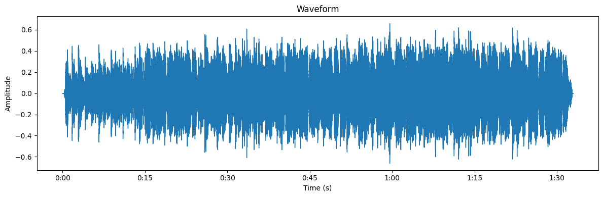
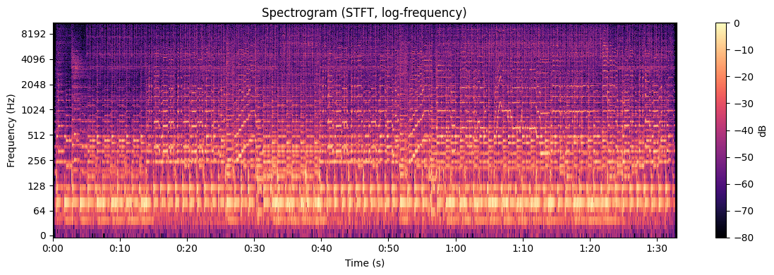
Once the audio is cleaned up, it can be the source for further analysis. A machine does not need to visualise sound to interpret it, but for the later examples, it can help to think about how the machine also starts with a waveform. As we have explored in earlier weeks, one of the basic ways to begin any audio analysis is to convert from the temporal domain (the waveform) to the spectral domain (e.g. creating a spectrogram using FFT).

Feature extraction¶

Feature extraction converts raw audio (waveforms or spectrograms) into compact descriptors that better reflect perceptual and musical structure. Features are commonly grouped by abstraction level:

• Low‑level descriptors are useful for timbre and energy tracking. They are typically short‑term and include features such as spectral centroid, bandwidth, rolloff, spectral flatness, RMS, and zero‑crossing rate.

• Mid‑level descriptors are useful for key, chord, and melodic analysis. They focus on harmonic/tonal relationships and include chromagram, constant que transforms (CQT), F0/pitch contours, and harmonic‑percussive decomposition.

• High‑level descriptors are useful for rhythm and structure analysis. They include temporal developments and include onset strength, tempogram, beat tracking, and segment boundaries.

Some of these work in the temporal domain (waveforms) while others in the spectral domain (spectrograms) and some use both in various combinations. It is important to remember that there is no easy way of determining any musical feature from a signal. For example, let us look at a chromagram, which is based on estimating the pitch classes from an audio recording:

From the chromagram, we see that there is a lot of chroma energy for E. This is also what the machine finds when calculating the average:

Let us then turn to another feature, trying to estimate the tempo of the song. We can begin by making a tempogram, which estimates prominent tempo profiles over time:

From this plot, it is not so easy to see what the estimated tempo is. However, if we ask the computer to smooth the signal and average across bands, we get a clearer result:

Notice how the instantenous tempo fluctuates quite a lot. This is not uncommon when dealing with real-world signals and is one of the reasons we typically average (“smooth”) the signal to find a result. In this case, the estimate tempo of 161 BPM is quite close to what humans would guess.

Source Separation¶

Source separation is the process of isolating individual instruments or voices from a mixed audio signal. This is a very challenging task and is still not completely solved. A very basic approach can be seen below where we split the signal into “harmonic” vs “percussive” components in the audio file:

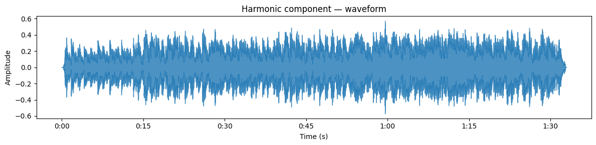
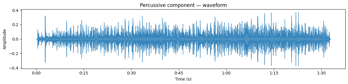
While traditional signal processing techniques have matured over time, it is the modern deep-learning approaches that can produce the best results.

Segmentation and event detection¶

Segmentation and event detection are processes based on locating boundaries and discrete events such as onsets, beats, or section changes. One of the traditional methods is based on looking at repeating patterns using a self-similarity matrix. Then the signal is compared to itself, and recurring patterns become visible:

The self‑similarity matrix shows pairwise similarity between frames, with repeating sections appear as off‑diagonal parallel stripes and boundaries appear where similarity across the diagonal drops. We can then ask the computer to (A) detect boundary times (change points) and (B) group frames into part labels (verse/chorus/bridge / repeated segments). This combination of local novelty (for transitions) and global clustering (for part grouping) is the standard practical route from an SSM to musical parts and transitions.

It is further possible to compare the segments to evaluate the musical form. However, this requires more code and interpretation, so we won’t consider that further here.

Music Information Retrieval¶

In the last example, we have transitioned from general machine listening and moved into the domain of music information retrieval (MIR), a specialized form of machine listening, aimed at extracting structured, actionable information from musical audio and related data. MIR combines signal processing, machine learning, music theory, and human-centred evaluation to support tasks such as metadata extraction, music search, analysis, learning, and interactive applications. The following sections describe core MIR tasks, typical approaches, and practical considerations for building and evaluating systems.

MIR tasks¶

• Classification and recognition includes identifying instruments, genres, or whether a recording contains speech or music. When working with large music collections, this means tools that can tag files, find similar pieces, or detect instrumentation in recordings. Methods range from simple spectral/timbral feature matching to modern neural classifiers. Common pitfalls are dataset bias, noisy recordings, and confusion between timbrally similar instruments.

• Recommendation systems combine audio‑derived features (timbre, tempo) with user behaviour to suggest music. Content‑based recommenders use the audio descriptors themselves. Collaborative methods exploit listening patterns across users. Many modern systems are hybrid and combine information from audio and user data. These systems help discover repertoire or playlists but are prone to bias and may have privacy concerns.

• Automatic transcription systems convert audio into symbolic scores (MIDI, MusicXML). Monophonic pitch tracking is quite stable these days, but full polyphonic, multi‑instrument transcription remains a challenge. Techniques include spectral analysis with onset/pitch heuristics, probabilistic sequence models, and end‑to‑end deep networks.

• Segmentation and structure analysis help find meaningful regions (intro, verse, chorus) or discrete events (onsets, section boundaries) in audio files. Approaches use self‑similarity and novelty detection, supervised boundary detectors, or learned embeddings. These tools are useful for form analysis, remixing, and practice. However, “meaningful” boundaries are often subjective, so evaluation uses tolerance windows and human judgement.

• Question‑Answering systems let you query audio with natural language (e.g., “Find tracks with a trumpet solo” or “show passages in major mode with fast tempo”). They combine audio tagging, metadata, lyrics, and semantic embeddings to match queries to segments. Key issues are building accurate multimodal indexes, mapping user language to reliable musical labels, and providing interpretable results.

• Mood, emotion, and other higher‑level feature extaction are active research topics in the MIR community. These revolve around estimating human responses to various types of music, which is also where they cross paths with contemporary music psychology research. This is challenging, given the large individual differences between people and the impact of cultural background and contextual factors.

Music Data¶

Data is at the core of any information retrieval system. Traditionally, MIR tasks primarily worked with symbolic data, in the form of MIDI or MusicXML files. The last decades, most research has been conducted on audio files, which can be seen as a form for subsymbolic data since it does not deal with “symbols” but with raw audio files.

Additional information can be found in metadata, including contextual information, such as artist or album details. Paradata can provide additional information about how the data was recorded or analysed, while user data can provide personal information about how people access and use the data, such as listening patterns and preferences.

For researchers, one major challenge is obtaining access to diverse music data while respecting legal and ethical constraints. Copyright, performer and composer rights, licensing terms, and privacy (for user or performer data) restrict what can be downloaded, redistributed, or used for training and publication. These constraints affect dataset size, representativeness, and the ability to share reproducible code and trained models.

To overcome some of these challenges, researchers often prefer openly licensed resources (CC0/CC‑BY, public‑domain) and well‑documented research datasets and always record and publish licence/provenance for each item used. Another solution is to not work with source material but rely on metadata or derived representations (e.g., spectrograms, embeddings) when raw audio redistribution is restricted. This reduces legal risk, improves reproducibility, and makes it easier for others to build on your MIR work while respecting creators’ rights and listeners’ privacy.

“Multimodal” MIR¶

Multimodal MIR combines audio with other data modalities to build richer, more robust musical understanding and retrieval systems. It complements audio-only signals (for example, lyrics can disambiguate mood or semantics, scores/MIDI provide exact pitches and timing, and video or motion reveal performer gestures or instrument identity), improves robustness and coverage by allowing missing or noisy audio to be recovered from aligned metadata or symbolic cues, and enables novel tasks such as audio–lyrics alignment, score-informed transcription, music‑video scene understanding, cross‑modal search (e.g., “find the clip where the singer sings ‘…’”), and richer recommendation.

Common data types that are used include:

• Audio (waveform, spectrograms, features)

• Symbolic (MIDI, MusicXML, scores)

• Text (lyrics, tags, reviews)

• Video / images (music videos, performance recordings)

• Metadata & interaction logs (artist, playlist co-occurrence, play counts)

• Sensor / motion capture (gesture, conductor data)

Practical multimodal MIR raises several recurring issues. Temporal alignment is critical: different modalities (audio, score/MIDI, lyric timestamps, video frames, motion capture) have different sample rates and may suffer timing jitter, and even small mis‑alignments can break tasks like score‑informed separation or lyric‑to‑audio alignment. Use robust alignment methods (dynamic time warping, score‑to‑audio alignment, timestamp correction) and always inspect results both visually and by ear.

Modalities are often missing or noisy in real systems, so design graceful fallbacks and robustness strategies: support audio‑only operation when other channels are absent, apply masking or imputation strategies for missing signals, and train models to cope with incomplete inputs so performance degrades gracefully rather than catastrophically.

Combining modalities increases compute and model complexity. Mitigate this by reusing pretrained embeddings, keeping fusion layers lightweight, and training modular subsystems (separate encoders with a small fusion head) so you reduce training cost and simplify ablation and debugging.

Evaluation must reflect both per‑modality performance and the end task: combine modality‑specific metrics (onset/offset F1 for transcription, SDR/SAR for separation, mAP for retrieval) with perceptual and user‑centred tests (listening studies, classroom tasks) to measure real usefulness beyond numeric scores.

Legal and ethical constraints matter throughout: lyrics, videos, and commercial recordings carry copyright and privacy limits. Prefer openly licensed datasets when possible, publish provenance and licenses for every item used, and consider sharing derived representations (spectrograms, embeddings) instead of raw audio to reduce legal risk and improve reproducibility.

Students will recognize concrete examples: score‑informed source separation (which requires tight audio–MIDI alignment), lyrics‑aware snippet search (which needs reliable text timestamps and robust handling of missing or incorrect lyric lines), music‑video analysis / visual beat tracking (which depends on accurate A/V sync and can be compute‑heavy), and recommendation systems that fuse audio with interaction logs (which raise privacy and fairness questions).

Practical workflow tips: start with one strong modality (usually audio) and add others only when they demonstrably improve the task; introduce modalities incrementally and run per‑modality ablation studies; use pretrained encoders or embeddings to reduce training cost; log and document data provenance and licenses for every source; and validate improvements with both objective metrics and simple listening tests or classroom evaluations.

Artificial Intelligence (AI)¶

Artificial Intelligence (AI) is commonly used to describe machine systems that perform tasks that normally require human cognitive abilities, such as perception, learning, reasoning, planning, and natural‑language understanding. In music, this includes systems that can both compose, perform, and analyse music.

Rule-based vs Learning-based systems¶

Although learning-based systems are what people talk most about these days, in general, we can talk about two main types of AI-based systems: rule-baesd and learning-based. There are also some exciting hybrid approaches.

Rule‑based systems rely on deterministic signal‑processing heuristics—peak picking, thresholding, spectral rules and simple decision logic—to make decisions. They are compact, easy to interpret and tune, and well suited to low‑latency, resource‑constrained tasks such as onset detection, simple VAD, or rule‑based beat tracking. Their disadvantages are brittleness to noise and domain shifts, extensive hand‑tuning, and limited ability to capture complex, data‑driven patterns.

Learning‑based approaches span classical supervised models (SVMs, random forests) on hand‑crafted features to modern end‑to‑end deep architectures (CNNs for timbre/scene classification, RNNs/TCNs for temporal structure, transformers for long‑range context). Self‑ and semi‑supervised pretraining (contrastive or predictive objectives) are common when labeled data are scarce, followed by task‑specific fine‑tuning. These methods typically offer higher accuracy and adaptivity, but require more labeled data or compute, can be harder to interpret, and demand careful validation against domain mismatch and dataset bias.

Hybrid approaches combine analytical signal‑processing priors with learned components to get the best of both worlds—for example, using handcrafted onset detectors to propose events that a learned model refines, applying learned post‑filters to classic spectrogram estimates, or enforcing musically motivated constraints (tempo, harmonicity) on ML outputs. Hybrids often improve robustness and sample efficiency while preserving some interpretability; a practical workflow is to start with a simple rule‑based baseline, then introduce learned or hybrid components where data and performance needs justify the added complexity.

Models¶

Some of the more well-known models you can come across in music research literature include:

• Hidden Markov Models (HMMs) are probabilistic, generative sequence models that represent latent states and state transitions; they are useful for producing interpretable event or state sequences (for example, note or phoneme sequences) and work well in low-data regimes. Their strengths are being lightweight, well‑understood, and providing explicit temporal‑state structure, while their limitations include limited capacity for long‑range dependencies and difficulty modeling complex, high‑dimensional observations.

• Recurrent Neural Networks (RNNs) and Long Short‑Term Memory (LSTM) networks process sequences step‑by‑step, with LSTMs using gating mechanisms to mitigate vanishing/exploding gradients and capture longer dependencies; they are widely used for frame‑level labeling, sequence‑to‑sequence tasks, and modeling expressive timing. Their advantages include good modeling of moderate temporal context and dynamics, whereas sequential computation can limit throughput and increase latency compared with more parallelizable architectures.

• Temporal or dilated convolutional networks (temporal CNNs, TCNs) use causal, time‑respecting convolutions often combined with dilated convolutions to model long histories in parallel; they offer large receptive fields with efficient, parallelizable computation and can be designed for low‑latency streaming. Pros include parallel inference and controllable receptive field size; cons include sensitivity to architectural choices (dilation rates, kernel sizes) which determine required context and memory usage. See also convolutional neural network.

• Transformers and attention‑based models use self‑attention to model arbitrary pairwise interactions across a sequence, excelling at very long‑range dependencies and sequence‑to‑sequence tasks such as transcription or structural analysis when paired with spectrogram or learned front‑ends. They often achieve state‑of‑the‑art results and provide flexible context modeling, but incur high compute and memory costs (quadratic attention can be expensive for long audio), though sparse/efficient attention variants can mitigate this.

Realtime vs non‑realtime¶

Machine listening systems can operate in different time modes; the choice strongly affects algorithm design, latency, and evaluation.

• Realtime (online) — Processes audio as it arrives and must keep latency small and predictable (latency ≈ window_duration + model_lookahead + processing_time; e.g., n_fft=2048 at sr=22050 → window ≈ 92.9 ms, hop=512 → 23.2 ms steps). This requires causal algorithms (causal filters, causal convolutions, stateful RNNs/TCNs, or streaming transformers with limited lookahead), a streaming frontend with short windows/small hops, and cheap incremental features (onset strength, low‑band log‑mel, incremental CQT) plus simple online post‑processing (peak picking, adaptive thresholds). Design priorities are low and stable latency, robustness to noise and jitter, and predictable, bounded compute so deployment constraints (CPU/GPU, battery, I/O) are met—practically this often means using lightweight models or hybrid pipelines (rule‑based front end + small learned model).

• Non‑Realtime (offline / batch) — processes full recordings after capture. Key trade‑offs: no strict latency, so you can use larger windows, global context, and bidirectional models (bi‑RNNs, full attention) for higher accuracy; able to run expensive post‑processing (Viterbi smoothing, global segmentation, search) and use entire‑track normalization/augmentation; better for high‑quality transcription, structure analysis, dataset annotation, or training‑data generation.

• Hybrid/buffered operation — a common compromise is to run a low‑latency online pass for immediate feedback and a higher‑quality offline pass to refine results; use short lookahead buffers (a few frames) to improve accuracy while keeping latency controlled, and document/expose the buffer size as the system’s lookahead.

Design decisions should be driven by the application: live interaction needs minimal, predictable latency and causal algorithms; analysis and annotation can exploit full-context offline methods for higher fidelity.

Examples¶

There are many practical examples of machine listening and MIR in both research and industry. Below are curated open‑source projects followed by some commercial examples.

Machine vs human listening¶

Human (music) psychology and machine listening/technology form a mutually reinforcing loop: psychological knowledge constrains and guides algorithm design, while technology supplies tools, data, and interventions that extend what we can measure, model, and apply. Key points and practical implications:

How music psychology informs technology¶

Perceptual representations derived from psychoacoustics—such as mel and ERB scales, loudness models, and masking curves—inform feature design and loss functions so that systems weight signal components in ways that match human sensitivity; this yields better compression, perceptual losses, and salience-aware processing.

Human temporal integration, memory limits, and expectancy shape choices for window and hop sizes, context length, and model architecture. Knowing how listeners integrate information over time helps decide whether to use short receptive fields, longer temporal context, or attention mechanisms to capture the appropriate temporal framing for a task.

Clear task definitions and annotation schemes benefit from psychological constructs: labeling targets in terms that reflect perceived categories (e.g., emotion, groove, perceived key) produces datasets and objectives that align with human judgments rather than with low-level signal properties, improving model relevance and interpretability.

Evaluation practice is guided by listening-based methods: objective metrics should be calibrated against perceptual judgements using listening tests (MUSHRA, pairwise comparisons) so that measured improvements correspond to meaningful changes for users; psychological methods help design rigorous, reliable perceptual evaluations.

Interaction and UX design draw on models of attention, affordance, and mental workload to produce interfaces and feedback that match user expectations. Insights from music psychology guide how to present analysis, how much detail to expose, and how to scaffold tasks such as practice tools or tutoring so they are cognitively effective and engaging.

How technology supports music psychology¶

Technology enables scalable data collection and analysis by providing audio repositories, crowdsourcing platforms, and annotation tools that make it feasible to gather large behavioural datasets and diverse stimuli. These resources support robust, ecologically valid studies by broadening the range of musical examples and participant populations that can be analysed.

Precise stimulus control and replication are made possible through synthesizers, signal‑processing toolkits, and digital audio workstations (DAWs). These tools let researchers generate tightly controlled stimuli to isolate perceptual variables, run repeatable manipulations, and share identical materials across labs for reproducible experiments.

Instrumentation for measurement—such as EEG, MEG, fMRI, motion capture, eye‑tracking, and physiological sensors—provides objective access to neural, motor, and autonomic responses to music. Combined with careful experimental design, these modalities allow researchers to link behavioural effects to underlying physiological processes and to explore timing, localization, and dynamics of musical perception and action.

Computational models and simulation expand the theoretical toolkit: machine learning and formal modelling enable quantitative hypotheses (predictive coding, attention models), permit in silico testing of ideas, and can simulate listener groups or clinical conditions (for example, hearing loss). These approaches help formalize perceptual theories and generate testable predictions for empirical work.

Finally, technology supports translation of psychological insights into real‑world interventions and applications. Examples include adaptive tutoring systems, hearing‑assistive signal processing, music‑therapy apps, and context‑aware recommendation engines that operationalize lab findings into tools with practical impact.

Some considerations¶

Feature design should be grounded in auditory perception: representations such as mel‑spectrograms, ERB‑based filters, and perceptual weighting derived from auditory filterbanks or loudness models produce features and loss functions that better align with human hearing. Using perceptually motivated front ends (and perceptual distance measures) helps models focus on signal components that matter for listeners rather than on raw signal energy alone.

Evaluation must combine signal‑level and perceptual assessments. Metrics like SDR, SIR, and SI‑SNR quantify numerical separation quality, but they do not capture perceived artifacting, timbral distortions, or musicality. Complement objective scores with small, well‑designed listening tests (MUSHRA or pairwise comparisons) to ensure measured improvements translate to audible benefits.

Adaptive and interactive systems benefit from psychophysical and motor‑learning models. Practice apps that are tempo‑ and beat‑aware can scaffold synchronization and entrainment by adapting difficulty, feedback timing, and metrical emphasis based on models of human timing and motor adaptation. Human‑centred design improves engagement and learning outcomes compared with purely automatic scoring.

Clinical and rehabilitative applications should tightly integrate perceptual and behavioral science with signal processing. Examples include music‑based gait training, auditory training tools, and cochlear‑implant signal‑processing strategies that are informed by listening studies and motor/cognitive constraints. Clinical claims must be validated with appropriate trials and domain expertise.

Validate features and objectives against human judgements before extensive optimisation on signal metrics. Start from perceptual baselines—confirm that chosen features or loss functions correlate with listener responses—and only then iterate on algorithmic improvements. Use mixed evaluation protocols that combine quantitative metrics with targeted listening studies or crowdsourced judgements to detect regressions that matter to users.

Ethical and cultural considerations¶

Make stimuli and datasets ecologically valid. Include diverse musical styles, real recordings (not only synthetic stimuli), and contextual cues so that models generalize beyond narrow laboratory conditions. Design experiments and datasets to avoid overfitting to artefacts of studio recordings or annotation conventions.

Document provenance, consent, and licensing, and keep humans in the loop. Record dataset licences, participant consent, and known limitations for reproducibility and ethics. Interactive workflows (active learning, human‑in‑the‑loop tuning, and iterative evaluation) often produce more useful and trustworthy systems than fully automatic pipelines.

Perception and meaning are culturally conditioned—models trained on narrow corpora may misrepresent or marginalize musical practices.

Privacy and consent matter when using user logs or physiological data; prefer anonymized, consented datasets and report provenance.

Be cautious about medical or therapeutic claims; collaborate with domain experts and validate clinically.

Bridging music psychology and technology yields systems that are both effective and meaningful: psychology grounds what we should measure and predict; technology scales, implements, and tests those hypotheses in real-world systems.

Questions¶

1. What is machine listening and what are the main stages of the signal→symbol pipeline?

2. Name three common audio preprocessing steps and their purpose.

3. Give three types of features used in MIR?

4. What is the difference between realtime (online) and non‑realtime (offline) processing?

5. Mention at least one popular Python library for machine listening.