Validating data

Motion data fails quietly. A dropped optical frame written as a coordinate triplet of zeros, a timestamp column that steps backwards, a documented sampling rate that is not the real one. None of these raises an error, and all of them produce a plausible number. The characteristic failure is not a crash but a believable wrong answer, so the only defence is a check that runs every time.

micromotion.validate is that set of checks. Each one exists because the failure it catches has occurred in real deposited datasets and gone unnoticed. The figures quoted below are measurements from those cases, given so that a reader can judge whether a tolerance is reasonable rather than take it on trust.

Using it as a gate

from micromotion import validate

findings = validate.validate_series(xyz, t=timestamps, documented_hz=200.0, where="A0001:P01")
validate.raise_on_error(findings)      # refuse to build on anything at "error"

validate_series runs whichever checks apply and returns a list of Finding objects, each with a check, a severity of "error" or "warning", a message and a where. Treat errors as build-stopping and warnings as facts to record in a manifest beside the number they affect.

Set expect_positions=False for a sensor whose output may legitimately be zero on every axis at once.

The checks

zero_triplets—gaps read as positions

Several optical systems, including Qualisys, write a dropped frame as 0.000 0.000 0.000. In laboratory coordinates that is a point on the floor, often more than a metre from where the marker actually is, so a reader that takes it literally sees the marker leave and return.

A median barely notices. Anything that sums or integrates does: in one recording, 93 such frames out of 118 698 gave a head marker a path length of 119.8 m where the true figure was 11.0 m, which is a factor of eleven from 0.08 % of the samples.

Exact zeros on all axes at once do not occur in real optical data, so the default tolerance is zero.

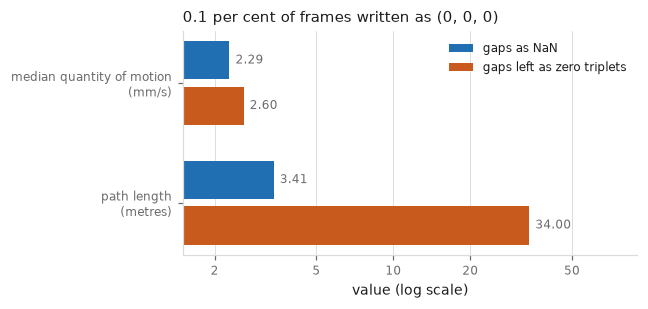
The figure is mm.path_length and mm.qom on the same synthetic recording twice, once with nine short runs of gap frames left as (0, 0, 0) and once with them set to NaN. One tenth of one per cent of the frames multiplies the path length by ten and moves the median by fourteen per cent, which is the asymmetry the check exists for: a robust statistic hides the defect that destroys every summing measure beside it.

implausible_position—the gap that is not a zero

zero_triplets catches a dropped frame written as three exact zeros. It cannot catch the near miss: a reconstruction that lands close to the laboratory origin without being exactly on it. Those samples are ordinary finite numbers and pass every sentinel and finiteness test.

mm.validate.implausible_position(marker_xyz)

The test is physical rather than statistical. A marker on a standing body stays within a band around its own median height, so anything below a third of it, or above two and a half times it, is a tracking artefact and not a posture. Markers whose median height is not a standing height, such as feet and floor references, are skipped, since there is no expectation to test them against.

Across 1018 optical person-recordings this fired twice. One placed a head marker 139 mm below the floor for 63 samples, and the other put one at 491 mm where its median was 1716.

Why so few matters so much

Those 63 samples are 0.5 per cent of the recording, and the median quantity of motion barely registers them. The spatial measures do not survive at all: the sway extent of that recording reads 977 mm where the true figure is about 48. Robustness is a property of a statistic and not of a dataset, so a defect that a median ignores can still be the whole of what a range, an area or a path length reports.

marker_average—a gap that survives averaging

The check above is not enough on its own, because of where the repair usually happens. Pipelines tend to repair gaps at the end, on the series they are about to measure. That is correct until you average several markers into one position, a "head" built from three head markers say, because the average destroys the evidence on the way in. The mean of two real coordinates and one zero triplet is a perfectly finite point, and no later gap check will ever flag it.

mm.validate.marker_average({"HF": hf, "HL": hl, "HR": hr})

The damage is a clean multiplicative bias, because markers on one rigid segment move together. With n markers of which k carry no data, the averaged position moves at about (n - k) / n of the true amplitude, and any speed derived from it is understated by the same factor. One dead marker out of three is exactly two thirds, which is a third less motion reported without complaint.

Partial gaps are worse in the opposite direction. Each gap frame drags the average a third of the way to the origin and back, which is a spurious excursion of roughly half a metre for a standing head, so the measure is inflated wherever the gaps are.

This is not hypothetical. In one 86-session collection, 22 files had head-marker gaps and four had a marker that was never tracked at all. Correcting it moved 19 of the 86 by more than half a per cent, the largest by 79 per cent, and collapsed the tail: the maximum quantity of motion fell from 38.9 to 15.2 mm/s and the 99th percentile from 24.7 to 12.7.

Why it went unnoticed for years

The median across that collection moved from 5.38 to 5.45 mm/s, which is about one per cent. A robust statistic is robust to this too, so the headline number looked stable the whole time while individual recordings were wrong by a factor of two in both directions. If you average markers, check them; do not infer from a steady median that nothing is wrong.

Repair each marker to NaN first, then use nanmean:

stack = []
for x in (hf, hl, hr):
    x = np.asarray(x, float).copy()
    x[(x == 0.0).all(axis=1)] = np.nan
    if np.isfinite(x).any():
        stack.append(x)
head = np.nanmean(np.stack(stack), axis=0)

finite_fraction and longest_finite_span—a series emptied by its own filter

A gap running off the start or end of a series cannot be interpolated: there is nothing on the far side to interpolate from. A band-pass then spreads the surviving NaN across the whole recording, and the result is indistinguishable from an absent sensor unless something checks.

start, n = validate.longest_finite_span(xyz)   # what to measure over instead

Measuring over the longest clean span, and recording how long it was, is usually better than either dropping the recording or silently closing the gap, since closing it makes the series claim a duration it does not have.

timestamps—a clock that is not a clock

Sorting a timestamp column into order is the tempting repair and the wrong one. It destroys the evidence that the clock misbehaved while leaving samples in an order the sensor never produced. One balance-board dataset carries 123 111 duplicate timestamps and 83 that step backwards; those are a device fault to be recorded, not a sort key.

rate_agreement—the documented rate against the measured one

Measure the rate, do not read it. Across one multi-device corpus, documented rates were wrong by up to 4.4 per cent, one was out by a factor of 37, and one set of wearable accelerometers ran at 191.29–207.73 Hz against a nominal 200. The true rate is a property of the individual unit, so participants sharing a device shared a clock and everyone else did not.

Every frequency-domain measure scales with this, and nothing further downstream can detect it, which is why it is raised as an error rather than a warning. See sampling rates for why measured_rate counts samples over the elapsed span instead of inverting the median interval.

frame_count—the 16-bit ceiling

C3D stores its frame count in a 16-bit field, so a conversion through C3D stops at 65 535 frames and says nothing. At 200 Hz that is 327.7 s of a 360 s recording: complete-looking, with the last thirty-two seconds gone. Treat a frame count of exactly 65 535 or 65 536 as a bug rather than a coincidence.

held_samples—a stored rate above the sampled rate

A sensor sampled below the rate it is written out at appears with each value repeated. The file then claims a rate the data does not carry, and any spectrum computed at the stored rate is wrong above the true Nyquist frequency. Some phone loggers write a row whenever any sensor updates, which produces exactly this.

duplicate_files—the same recording twice

Found by content rather than by name, because the usual cause is a rename that left the original behind under a name no manifest mentions.

What no check here will catch

Six failures from real use, none of which this module can see, all of which produced a believable answer.

A unit that is recorded and then ignored. A derived table carried unit per row and a consumer hardcoded unit="g", inflating one collection by 9.80665. Nothing was missing or malformed; the wrong constant was simply applied. Read units from the data beside the numbers, and print a median in physical units where a human will see it. Quiet standing is a few mm/s, and a figure in the tens is telling you something.

A group mean that counts markers that were not visible. A group average taken over every marker at every frame counts an occluded marker in the divisor, and since band_limited_qom interpolates gaps, that marker contributes a near-zero speed rather than nothing at all. The number then tracks camera coverage rather than movement: 16 to 17 per cent low on a realistic dropout pattern, with the speed series correlating up to +0.70 with the per-frame count of visible markers. group_qom defaults to normalize="visible", which excludes each marker where it was absent; normalize="worn" performs the older computation, for reproducing a figure that used it. Nothing in this module could have seen it, because every individual trajectory was valid; the fault was in how they were combined. validate.marker_average documents the same bias one level up, for spatial averaging.

A rank statistic hiding a scale error. When that bug was found, every Spearman correlation in the affected analysis was unchanged, because rank statistics are invariant to multiplication by a positive constant. A pipeline reporting only correlations is not checking its own scale.

Silent emptiness. A glob returning zero files after a folder was restructured; a second after an extension was renamed; a join matching 1616 of 30639 rows because two files spelled a track name differently. Each carried on and produced a smaller, plausible result. Assert the counts you expect after every glob and join, with len(files) == n_expected and merged.shape[0] == left.shape[0], and fail rather than continue.

A reliability statistic that certified an artefact. A jerk value was computed on a channel whose sensor could not carry the band it was computed at, a 100 Hz grid over a 15 Hz sensor. Split-half reliability, first half of a recording against the second, came out at 0.983: the second highest of any collection, and it was read as evidence that the measure was not amplified noise. It was reliability of the upsampling. Interpolation is deterministic, so its artefacts repeat perfectly between the halves of a recording; the honest value from a channel that could carry the band was 0.909, i.e. lower. Reliability tells you a measure is stable, not that it is measuring the thing you named it after, and a deterministic artefact is the most stable thing in any pipeline.

An odd-against-even-windows statistic within a recording does not share this failure mode, since interpolation kinks contribute equally to both halves. Report both when the question is whether a derivative is real.

A conclusion written as a constant. One script printed (flat -> NO habituation) and titled its figure FLAT ... (no habituation) as literal strings, whatever the statistics came out as. They came out r = −0.114, p = 0.038, and the same number was cited elsewhere in the same project as evidence for the effect. Both files were right about the arithmetic and the disagreement was invisible, because re-running the script could never change the sentence. Derive verdict text from the value, always.

A deliverability check enforced in only one place. A scan computed a wideband jerk for every recording whether or not its rate could carry the band, leaving the gate to the consumer. The obvious consumer filter, "the value is not null", silently readmitted every recording the gate was meant to exclude. Enforce deliverability where the value is produced and where it is consumed; a null is not the only way to say "not measurable", and it is the easiest to lose.

The pattern across all of these is the same, and it is the one this module exists for. The dangerous failure is not the one that raises, it is the one that returns something reasonable.

Is it standstill throughout?

A recording of stationary behaviour should contain stationary behaviour and nothing else. In practice recordings are trimmed by hand, or not at all, and what survives at the edges is participants walking into position, settling, stepping onto a force plate, or reacting to being told the recording has ended.

speed = mm.speed_from_position(xyz, fs)
validate.edge_motion(speed, fs)          # which end, and by how much
validate.settling_time(speed, fs)        # (head, tail) seconds to trim

The comparison is against the recording's own settled interior rather than an absolute threshold, because the quantity spans two orders of magnitude across sensor types.

This is worth checking even when you believe the trimming was done. Across 1465 recordings in one corpus, 784 were clean and the rest were not. Two collections accounted for nearly all of it, and one recording ended at 1608 mm/s against a settled 3.06, which is someone walking away inside a dataset described as standstill.

settling_time answers the follow-on question rather than leaving it to a guess. One collection trimmed a fixed twelve seconds to remove a synchronisation clap; measured, the settling ran to twenty-five seconds at the median and thirty-five at the ninetieth percentile, and correcting it changed a published null result into a significant effect.

A ratio test needs an absolute floor

On a near-motionless reference marker a ratio is meaningless, since twice a settled level of 0.1 mm/s is still nothing. If you act on edge_motion automatically, require an absolute speed as well as a ratio.

Repair at source, or on read?

When a check fires on archival data you have two options, and the right one depends on what depends on the file.

Repair on read if the recording backs a publication, or if deposited code reproduces published figures from it. Rewriting such a file breaks the reproduction, and a gap encoding that is documented is not a defect even when it is a hazard, since it may be the convention that the published analysis code expects.

Repair at source if the encoding is undocumented, nothing computes from the file yet, or the stored values are wrong rather than merely awkward.

Either way, record what was found. A dataset that documents its own hazards is more useful than one that has quietly removed them, because the second gives a reuser no way to tell whether a number they compute matches the published one.