The four bands

There are four quantity-of-motion conventions here and they are not interchangeable. Reporting a number without saying which one produced it is the single most common way results in this field stop being comparable. The four are named in mm.BANDS and are passed to qom by name, as band="micromotion", band="wideband", band="noresp" or band="optical_legacy".

micromotion—0.2 to 5 Hz

A band-pass, and the package default, exported as mm.BAND. It is the only convention that can be applied to every sensor, so it is the one any cross-collection comparison must use.

The lower edge is where inertial devices stop agreeing with each other

BAND was chosen by a sweep across seven optical datasets, and it serves optical data well. On INERTIAL data its lower edge is also the point at which different devices stop measuring the same quantity, which is a separate fact and a sharper one.

Measured on four accelerometers mounted in one stack on one chest — so the body, the moment and the placement are all held fixed — against optical markers on the stack itself:

lower edge	spread across the four devices
0.2 Hz	9.2x (from 3.6 to 32.6 times the optical truth)
0.5 Hz	1.2x (from 1.9 to 2.3)

Almost the whole disagreement between devices lives below 0.5 Hz. Quantity of motion integrates acceleration and integration divides by frequency, so a device that misbehaves only at 0.3 Hz misbehaves badly. The worst of the four carried 62 times another's power at 0.2–0.5 Hz and 0.6 times it at 2–5 Hz — the noisiest device in the band and the quietest above it.

This is not an argument for moving BAND. It is an argument for STATING the lower edge beside any inertial figure, and for expecting cross-device comparisons at 0.2 Hz to be dominated by whichever device drifts most.

noresp—0.45 to 5 Hz

Exported as mm.NORESP_BAND: the canonical band with its lower edge raised above respiration.

On a chest-worn sensor the 0.15–0.45 Hz stretch that BAND keeps is dominated by respiratory chest tilt. The ribcage turns the sensor as it expands, so what the accelerometer reads there is gravity re-projected between axes — a rotation, not the sensor travelling. Measured across the year-long chest-phone record, 94 to 99 per cent of the power in that band lies perpendicular to that day's gravity vector, implying a tilt of 0.05 to 0.14 degrees. So a BAND value from a chest sensor carries a respiratory term inside every number, and a noresp value does not.

The choice between the two is a purpose decision, not a correctness one. For a cardiorespiratory torso measure, and for any comparison with the rest of the corpus, use BAND: the respiratory term is part of what is being measured, and it is the band everything else was computed at. For micromotion above respiration — a postural question asked of a chest-worn sensor — use noresp, and say so. The StillStanding365 record deposits both, as qom_mm_s and qom_045_5hz_mm_s, each with its band stated, which is the practice to copy.

It is not the compensated variant, which raises the edge further, to 0.5 Hz, and also notches the recording's own cardiac peak. noresp changes the band and nothing else; the ballistocardiac impulse is still inside it.

optical_legacy—10 Hz low-pass, no lower edge

Exported as mm.OPTICAL_LEGACY_BAND, which is (None, 10.0). It retains sub-0.2 Hz postural drift. For optical position that drift is real movement, and this is the convention behind most published standstill figures. Every band-limiting entry point accepts lo=None for it.

A value computed here is not comparable with one at BAND, and the gap is large. On one corpus, moving the lower edge from 0.3 Hz to 0.2 Hz alone raised per-marker levels about ten per cent; removing the lower edge entirely raises them much further, because on an accelerometer roughly half the velocity power sits below 0.3 Hz. Reporting a legacy-band figure beside a canonical-band one without saying which is which is the most common way this corpus has produced an apples-to-oranges comparison. One report quoted a three per cent agreement between two numbers computed at different bands and called it striking.

wideband—0.2 to 10 Hz

Exported as mm.WIDEBAND. It is for jerk and other high-derivative measures that need the octave the canonical band gives up.

Use it only where effective_band(fs) confirms the rate supports it, and never infer the rate from a file's grid, since a uniform grid may be an upsample of a much slower sensor, and this corpus contains 364 days where it is. A quantity computed here is not comparable with one computed at BAND, and is not computable at all on the slower collections.

Check deliverability where the value is produced and again where it is consumed. A scan that computes a wideband jerk for every recording regardless of rate, leaving the gate downstream, will be defeated by the obvious downstream filter: "the value is not null" readmits every recording the gate was meant to exclude. Carry the measured sensor rate alongside the value and test against it.

Deliverability is a property of a channel, not of a collection. A collection whose deposited channel cannot carry WIDEBAND may have a faster channel on the same device that can, as in the fusion discussion in Sampling rates. "This collection has no jerk" and "this channel has no jerk" are different statements, and only the second is usually true.

A bounded search returns its own boundary

Ask for the largest peak between two frequencies and you will always get an answer, including when there is no peak between them. What comes back then is a property of the band you drew rather than of the body you recorded. It does not raise, it is not a NaN, and it is a plausible number that goes straight into a mean.

The answer does not have to sit ON the boundary to BE the boundary. This is the part that keeps being missed, and it is why the failure survives being found. There are two symptoms and only the first is obvious:

symptom	what it looks like	what finds it
the answer sits on the edge	a column of values all reading exactly 6.0 breaths a minute, or exactly 0.7 Hz	a check for values piled up on an extreme
the answer is proportional to the edge	a spread of ordinary-looking values that happen to average 1.3 times the edge, none of them equal to it	moving the edge

The second is the common one on real data, and every equality check passes it. A spectrum that falls steeply has no maximum to offer except near the bottom of whatever band you drew, and the exact bin it lands in depends on the noise, the Welch grid and any filter you applied — so the values scatter, look like measurements, and move together when the band moves. Put a band-pass over the same band first and it is worse: the filter's rising skirt reaches inside the passband, so the largest surviving value sits a fixed fraction above the lower edge instead of on it.

This corpus has now met it five times. The sharpest case is a remote-photoplethysmography pipeline that band-passed a colour signal between 0.7 and 4 Hz and reported the largest peak inside. Over a year of daily recordings it returned 1.24 to 1.33 times its own lower edge; sweeping that edge from 0.5 to 1.5 Hz dragged the reported heart rate from 40 to 116 beats a minute; and it never correlated with a worn reference above 0.21 at any setting. None of its values sat on a boundary. The diagnostics it shipped with — the peak's height over the band median, the share of power in the band — predicted nothing, because on a falling spectrum the artefact scores well on both.

The test is to move the boundary

r = mm.band_edge_sweep(signals, fs, (0.7, 2.2))
r["follows"]     # True: the edge explains the answers better than a rhythm does
r["factor"]      # what multiple of the edge they sit at
r["r_max"]       # the best correlation against a reference, at any edge

A genuine rhythm returns the same frequency at every edge below it. An estimate that is the edge returns c times the edge at every edge. band_edge_sweep fits both hypotheses and reports which fits better, so there is no threshold to argue about, and it covers both rows of the table above — an answer sitting exactly on the edge is the same test with factor at 1.0. Pass a whole collection and a reference and the second question follows: if the estimate carries information about the body, it correlates with an independent measurement of the same quantity at some edge.

Two limits, both real. Push the swept edges above the rhythm and every estimator follows them, correctly, because the rhythm is no longer in the band — so keep the sweep below the frequency you expect. And the estimator is injectable, called as estimator(item, fs, (lo, hi)), precisely because the pipeline under suspicion is usually not a function in this package.

What this package's own finders do

Audited on synthetic 1/f series with nothing in a 0.7–2.2 Hz band:

function	median answer, as a multiple of the lower edge	exactly on the edge
mm.spectral_peak	— (returns NaN)	—
mm.cardiac_peak	1.05×	10 of 40
mm.dominant_frequency	1.07×	0 of 40
mm.instantaneous_rate	1.00×	0 of 40
mm.respiration_rate	1.41×	0 of 40

spectral_peak is the only one that refuses, and that is what require_peak buys: it asks whether the largest value is a local maximum of the spectrum divided by a log-log line fit across the band, and returns NaN when it is not. The other four are bare maxima and stay bare maxima, because published figures came out of them; since 1.12.0 they warn instead, naming the multiple. Note the bottom row: respiration_rate band-passes to the band it then searches, which is the shape that lands furthest from the edge and is therefore hardest to see.

Note also the third column. Three of the four never land on the edge at all, so an audit that looks for values piled up on a search boundary — which is what this corpus ran, and what found the first four instances — would have passed them without a word.

If you are writing the estimator

State the band beside every rate. Prefer mm.spectral_peak, which fails to NaN, and treat the count of NaNs as part of the result rather than a nuisance; a rate aggregated over many recordings under this rule is missing its weakest cases, and that is a fact about the aggregate. Where a bare maximum is what you want, say so with require_peak=False and know what you are asking for.

Two repairs that do not work, both tried and measured. Rejecting the edge bin moves the maximum to the next bin along: on one corpus 662 of 930 values on the edge became 198 of 268 one bin up. Raising a signal-to-noise threshold selects the artefact rather than excluding it, because the lowest bin of a falling spectrum has both the most power and the highest power-over-band-median of anything in a band drawn above the knee — tightening it from nothing to 5 took the share of days reading exactly the band floor from 21 per cent to 32.

A share of power needs both its bands named

A "fraction of power in band X" is a ratio of two integrals, and it moves when either band moves. Four published-looking figures for the share of standstill motion — 38, 43, 45 and 58 per cent — circulated in this corpus and were quoted against one another as though they measured the same thing. Traced to their origins, each came from a hand-rolled fraction with a different, sometimes unstated, denominator: the 58 traces only to its own 0.10–3.0 Hz denominator, where those bands read 59 under the arithmetic below, and the 45 is untraceable to any measurement at all.

mm.band_share(x, fs, num_band=..., den_band=...) is the arithmetic with the bands made mandatory and keyword-only, so a call site cannot leave either unstated. It raises when the numerator band reaches outside the denominator, warns when the denominator's upper edge exceeds what the rate can deliver, and warns on non-finite input. mm.band_share_from_spectrum is the same rule for a spectrum already in hand.

The three-label rule when quoting one: state the domain (power of what quantity), the site (sensor and placement) and both bands. Acceleration power and position power weight the spectrum by a factor of frequency to the fourth relative to each other, so a share of one is not even approximately a share of the other, from the same sensor on the same body.

And the arithmetic, which is the fourth label

Two bands on one spectrum still do not fix the number, because there are two ways to turn a Welch spectrum into a band power and this package used both before it said so. The rule is the quadrature — trapezoid, which weights the two edge bins by a half, or a plain sum of the bins in the mask, which is the rectangle rule and is what a "bin-summed fraction" means. The closure is what the edges mean — [lo, hi] or [lo, hi). Four combinations, four numbers.

They are not close. Measured on chest-accelerometer standstill recordings, holding the mask fixed so that only the quadrature rule changed, a respiratory share moved by up to 0.034 absolute on a share of about 0.16, over a fifth of the value; closure costs a further 0.025 absolute on the same recordings. Closure costs that much because analysts choose round band edges: at the conventional 60 s window the bins are 1/60 Hz apart, so 0.40, 0.70, 2.20, 3.0, 5.0 and 8.0 Hz all land exactly on a bin, and closing the interval adds a whole bin at the numerator's upper edge and another at the denominator's, which do not cancel.

The reason this stayed invisible is that the two agree exactly where the band is flat: the trapezoid's half-weighted end bins remove precisely one bin's worth, so trapezoid-over-[lo, hi] equals bin-sum-over-[lo, hi) on flat power. The disagreement is driven by the slope inside the band, so it is worst at the low end of a red spectrum — the respiratory band, on every body-worn sensor here.

Which is which, in this package:

Function	Rule	Closure	Denominator
mm.band_power, mm.band_power_fraction	trapezoid	[lo, hi]	whole spectrum (band_power_fraction)
mm.band_share, mm.band_share_from_spectrum	integrate=	interval=	named band, mandatory
mm.spectral_band_fractions	sum	[lo, hi)	named band, physio.DEFAULT_TOTAL_BAND if unset

band_share defaults to integrate="trapezoid", interval="closed", which is what it and band_power have always computed. band_share(..., integrate="sum", interval="half_open") reproduces spectral_band_fractions on the same spectrum to floating point, which is the call to use when extending numbers computed that way. Neither is more correct; only one of them is the one your comparison was computed under.

So the label is four things, not three: the domain, the site, both bands, and the arithmetic. In prose that reads "25 per cent of 0.2–5 Hz raw chest-accelerometer acceleration power lies at 0.8–2.5 Hz, integrated with the trapezoid rule over closed bands", and in a table it is a share_convention column reading trapezoid/closed or sum/half_open. A share is comparable only with a share computed the same way.

This corpus holds trapezoid/closed, the default above. Four analysis scripts that summed bins over half-open bands were carried onto it, which republished a chest-phone cardiac share from 58 to 59 per cent, a vest respiration figure from 16.6 to 15.1, a definitional fold from 3.1 to 3.2, and 18 of the 24 numbers in one decomposition table. That is a re-measurement rather than a refactor, and it buys one thing: every share in the corpus can now be quoted against every other.

Where a number should come from

Data, then toolbox, then report, then book. A figure in a paper should trace back through a report that called this package, to a deposited recording — and at no step should an analysis carry its own copy of something the package already does.

That is not tidiness. A copied estimator drifts, and the drift is invisible because both versions run without error. This package exists because a corpus of standstill analyses had, at various times, one script band-passing at 0.3 to 10 Hz while the rest used 0.2 to 5, another integrating with a cumulative sum where the rest used a trapezoid, and a third computing a device factor from a channel nobody else read. Each was defensible alone and wrong in company.

The most expensive instance so far: a report reimplemented resampling with a bare scipy.signal call and published that an optical head marker cannot show the two regions of postural control. It can, in 619 of 626 recordings. The private copy aliased, the estimator read the shortest lags, and the conclusion inverted. Nothing errored, and a plausible mechanical explanation grew on top of the artefact and made it harder to doubt.

So: if this package has a function for it, call it. If the function is wrong, fix it here, where one fix reaches every analysis — and where a test can hold it.

Why the lower edge is optional for position and mandatory for acceleration

An optical system measures position directly, so slow drift is a genuine displacement and keeping it is a choice.

An accelerometer cannot offer that choice. Gravity is a DC term, and integrating a signal with any residual offset produces a ramp that swamps the result. The package therefore raises on band="optical_legacy" for acceleration rather than return a plausible-looking number.

mm.qom(acc, fs, kind="acceleration", band="optical_legacy")
# ValueError: the 'optical_legacy' band has no lower edge, and an accelerometer
# cannot be integrated without one...

Why 0.2 Hz at the bottom

The lower edge was chosen by measurement rather than by convention. Swept across seven optical datasets and 665 recordings, the between-dataset spread is:

lower edge	spread
0.15 Hz	3.2 %
0.20 Hz	2.1 %
0.25 Hz	2.7 %
0.30 Hz	6.2 %
0.40 Hz	10.1 %

A clear optimum, and also where the 20 Hz origin dataset stops being an outlier in either direction.

The edge interacts with the statistic, which is easy to miss. At 0.2 Hz the median speed converges to 2.1 per cent and the mean only to 4.6; at 0.3 Hz it is the other way round. Report the median at this band. A mean here would be looser than what it replaced.

An edge this close to DC has to be checked against integration drift, since that is the failure it exists to prevent. It survives: on accelerometer data the mean-to-median speed ratio, which climbs when drift leaks in, is 2.07 at 0.2 Hz against 2.00 at 0.3, which is flat. The filter transient does lengthen to 40 seconds at each end rather than 27, so a recording shorter than about two minutes has no clean interior at all. That rules the band out for short trials; it does not affect standstill protocols, which run six minutes or more.

Why 5 Hz at the top

Because that is what the devices can deliver. A band above Nyquist is not a convention, it is a defect that returns a plausible number, and the ceiling has to be one every collection can support:

device	sampling	Nyquist	5 Hz?
phone, fused linear acceleration	~15 Hz	7.5	yes
optical, 20 Hz subset	20 Hz	10	yes
collaborators' audience data	10 Hz	5	at Nyquist
optical and inertial, rest	100–256 Hz	50–128	yes

A 10 Hz ceiling fails the first row on 354 of 355 days and sits exactly on Nyquist for the second, where it is silently clamped to 9.9.

The phone case is the instructive one, and it has two layers. Those files are stored on a 100 Hz grid, which is a six-fold upsample, so nothing above 7.5 Hz in them is real. The reason is not that the accelerometer is slow, since measured across the year it runs at about 50 Hz. The deposited channel is linear acceleration, which the logging app derives by fusing accelerometer, gyroscope and magnetometer to remove gravity, and a fusion runs no faster than its slowest input, which here is the 15 Hz gyroscope. So the constraint is the channel, not the sensor, and a pipeline built on the raw accelerometer channel would have roughly three times the bandwidth.

What the ceiling costs. Measured over 466 person-recordings from seven collections, computing both bands from the same array so that only the band differs. The typical recording barely notices—the median difference is 1.3 per cent, and 95 per cent of quiet-standing sway power lies below 1 Hz anyway—but this is a distribution, not a bound, and it has a tail:

collection	median	90th percentile	maximum
Championships (optical, 100–200 Hz)	2.83 %	5.66 %	9.07 %
Taqasim	1.66 %	2.67 %	4.16 %
Stillness2025	1.11 %	1.70 %	2.29 %
HpSp	1.10 %	3.05 %	5.32 %
Sverm	0.98 %	2.93 %	7.03 %
StillStanding365	0.61 %	1.79 %	2.38 %
all	1.28 %	3.24 %	9.07 %

Nineteen per cent of recordings exceed 2.3 per cent and the largest exceeds it fourfold, so the median is not a bound. The difference is largest exactly where the ceiling matters most: on the optical championships the median is above 2.3 per cent and 50 of 80 sampled recordings exceed it, because markers sampled at 100 to 200 Hz genuinely resolve the octave between 5 and 10 Hz, while a chest accelerometer that never delivered that octave loses nothing by giving it up.

Rankings survive this, since it is a small and fairly uniform shrinkage rather than a reordering. Quoted absolute levels do not.

What it costs that matters. Jerk is two derivatives higher and lives in the octave being given up: at 5 Hz it is 37 to 66 per cent of its 10 Hz value, and the ranking shifts as well. Jerk is therefore computed at WIDEBAND, on collections fast enough to deliver it, and nowhere else. On the phone collection the wider jerk was never real, and computing it there inflated the figure by 18 to 27 per cent with interpolation.

The nominal edge is not where the filter stops

A band written as 0.2–5 Hz does not pass everything below 5 Hz and reject everything above. It is a zero-phase fourth-order Butterworth, applied forward and backward, and it is rolling off well before its nominal corner. Measured on pure tones of known amplitude, recovering the analytic mean speed:

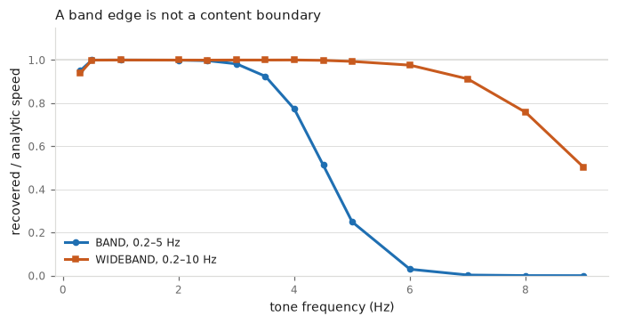
tone	canonical BAND 0.2–5 Hz	WIDEBAND 0.2–10 Hz
0.30 Hz	0.951	0.939
0.50 Hz	1.000	0.999
1.00 Hz	1.000	1.000
2.00 Hz	0.999	1.000
2.50 Hz	0.997	0.999
3.00 Hz	0.982	1.000
3.50 Hz	0.924	1.000
4.00 Hz	0.773	1.000
4.50 Hz	0.513	0.998
5.00 Hz	0.249	0.993
6.00 Hz	0.030	0.976
7.00 Hz	0.003	0.912
8.00 Hz	0.000	0.758

Read the 5.00 Hz row. A pure tone exactly at the canonical ceiling survives at a quarter of its true amplitude. Full fidelity, better than 99 per cent, extends only to about 2.5 Hz, so the usable passband is roughly half the nominal upper edge. The same holds at the bottom: 0.3 Hz already reads 5 per cent low, so content near the 0.2 Hz corner is heavily attenuated rather than passed.

Three consequences worth keeping in mind.

Do not read a band edge as a content boundary. Moving the ceiling from 10 Hz to 5 does not discard the 5–10 Hz octave; it discards, in effect, everything above roughly 3.5 Hz. That is why the jerk change is as large as it is.

Do not probe a filter at its own corner. A validation test that puts its test tone at the stated edge will fail against the analytic answer, and the failure is the filter working correctly. Probe inside the passband and characterise the roll-off separately, as here.

The steepness is a consequence of zero-phase filtering. filtfilt applies the response twice, which is what buys zero phase distortion. That matters when the output is going to be differentiated or integrated, and it costs a sharper effective roll-off than the nominal order suggests. The trade is deliberate, but the effective bandwidth is narrower than the label.

The edge is not modality-neutral

The sweep above is over optical datasets, and the accelerometer check above is about drift. Drift is not the only thing that moves. Holding the pipeline fixed and changing only the lower edge from 0.3 to 0.2 Hz:

recorded quantity	change in reported speed
position, optical marker	+7 to +18 %
acceleration, body-worn	+25 to +94 %

The asymmetry is structural. Speed comes from differentiating position and from integrating acceleration, so the operator converting the recorded quantity to velocity is multiplication by f in one case and division by f in the other. Measurement noise is roughly white in whatever the device records, which means the same sliver of extra low-frequency bandwidth is suppressed for a marker and amplified for an accelerometer. It is largest on chest-worn sensors, where 0.2 Hz sits on the respiration fundamental.

What follows:

• Rankings survive; levels do not. Where only the band differs, Spearman correlations stay at 0.94 and above. Comparisons of who moved more are robust to this. Comparisons of how many millimetres per second are not.
• State the band whenever quoting an absolute level from an accelerometer. The same recording supports two defensible numbers a factor of two apart.
• Treat cross-modality level comparisons as approximate, however harmonised the band. A shared band does not by itself make an optical and an inertial measure interchangeable.

What the difference costs

Measured on one championship edition, the band-pass reads 15.5 per cent below the low-pass on identical data.

The choice is not only about matching what is in print. Across seven independent optical datasets, covering two tracking systems, four sampling rates, twelve years and 789 recordings, the convergence is:

Convention	Spread across datasets
micromotion band-pass	3.5 % (median speed)
optical_legacy low-pass	5.9 %

The low-frequency drift the legacy filter keeps is the part that varies between datasets; the band-limited part is the part that does not. If an invariant is the claim, the band-pass states it better, and it is also the only convention under which an accelerometer can confirm it.

A trap at 20 Hz

The legacy low-pass cannot be computed at 20 Hz. Its 10 Hz cutoff is Nyquist there, so the filter has no transition band left. Compute legacy values at the native rate. This also means any dataset natively recorded at 20 Hz has always had its legacy figures computed at the edge of what its rate supports.

These definitions are duplicated inside archival records

Six deposited data records carry a hand-written copy of the band-pass, and some of them of the fourth-order derivative and the gap-bridging rule as well. That is deliberate: an archival record has to run for someone who has only that folder, so it may not import this package, and the definition is written out in numpy and scipy inside the record instead.

The consequence is a fork that nothing keeps in step. Changing BAND, ORDER, NYQUIST_MARGIN, the interpolation limit or the derivative rule here does not change those copies, and nothing fails: each record's own check imports its own generator, so the record stays internally consistent while drifting away from the corpus it belongs to. It is the same shape as a test holding its own copy of a constant, and it is invisible from either side alone.

A change to any of those constants is therefore a change to seven places, not one. The deposit tree carries deposited_vs_toolbox.py, which runs both implementations on the same synthetic signals and reports the worst disagreement; run it after touching filters, qom or resample.

Two conventions differ legitimately between records, and the check reports which each uses rather than enforcing one. Some pass acceleration in g and some in m/s², and some integrate with the rectangle rule while others use the trapezoid. The two quadrature rules differ by a fraction of a per cent—systematic rather than noise—which is why velocity_from_acceleration takes integrate rather than choosing for the caller.